Abstract
The log-logistic distribution has been widely used in survival analysis, particularly in modeling survival times and event data in healthcare and biological studies. This research employs the Maximum Likelihood Estimation (MLE) method to examine parameter estimation for the Log-Logistic Tangent (LLT) distribution. From the simulation study, it was evident that the estimated values of parameters β and α deviated from their true values. Specifically, the estimated value for β was 1.4291, while α recorded a value of 0.6698. Their respective standard deviations were 0.0733 (β) and 0.1512 (α), reflecting the variability across iterations. Further analysis of the LLT model’s asymptotic properties confirmed the consistency of the estimation process, as parameter estimates converged to stable values with increasing sample size. Additionally, standard errors and Fisher information were utilized to further verify the asymptotic normality of the estimates. To validate the LLT model, it was applied to real-world data, successfully yielding survival probability estimates. In conclusion, this study suggests improving the LLT model to reduce bias, exploring alternative estimation methods, and refining optimization techniques for better accuracy.
Keywords
Mixture Cure Models, Cure Models, Logistic Distribution, Modified Log Logistic Distribution
1. Introduction
Survival analysis is used in many applications when we want to know the amount of time before the considered event occurs. Survival analysis assumes that in a standard model all individuals are going to experience the event if there is sufficient time for observation. for example, if the event of observation is death due to some type of cancer. Sometimes time to event data is not observed (censored observations). The standard cure models makes an assumption that the cure status information is an unobserved (censored observations). Safari et al., used kernel methods to estimate conditional survival function, latency function and cure probability in the presence of cure status information.
In recent years, the application of cure models has gained prominence in survival analysis, particularly in oncology, where understanding long-term survival rates is crucial. This study focuses on the Log-Logistic Tangent (LLT) distribution, which offers a robust framework for modeling survival times in cancer patients
| [5] | Syn, N. L., Kabir, T., Koh, Y. X., Tan, H. L., Wang, L. Z., Chin, B. Z., & Goh, B. K. (2020). Survival advantage of laparoscopic versus open resection for colorectal liver metastases: A meta-analysis of individual patient data from randomized trials and propensity-score matched studies. Annals of Surgery, 272(2), 253-265. |
[5]
. By addressing the unique challenges associated with censored data and the presence of cured individuals, this research aims to enhance the accuracy of survival estimations in oncology studies. The significance of this study lies in its potential to inform treatment strategies and improve patient outcomes by providing reliable survival probabilities.
In survival analysis the subjects under study are said to be cured "not expected to experience the event of interest". Thus, the population is made up of a mixture of sub-populations; the cured subjects and the uncured subjects. In the field of medicine, blood cancer has been found out to be the most prevalence disease upon diagnosis. There are different types of infections for example the patients with bladder cancer have a ninety percent of bladder transitional cell carcinoma while the bladder stem cell carcinoma accounts for a percentage greater than five. However, the percentage may reduce depending on the pathological histology. Different lifetime models like log-logistic, Rayleigh, gamma, log-normal, and Weibull models have been used extensively in the medical field.
1.1. Problem Statement
In the recent years, health care has developed with the recent due to computational developments. The use of log logistic models has helped in the development mathematical statistics in the health care sector
| [4] | Vigas, L., Perez, J., & Rodriguez, M. (2021). Introducing the odd log-logistic Neyman type A long-term survival models. Journal of Biostatistics, 49(5), 301-320. |
[4]
. The cure models have been greatly used in the survival analysis. A fraction of the population is the statistically cured as the cancer free general population is they are subject to the same experience. The mixture cure models can be used greatly in estimating long term survival that is a requirement in the health economic evaluations. Cancer has put in some burden to the health care industry, patients, societies, and healthcare systems in the world. Some of the part of the country cancer has improved while in others it has been left to be a burden especially to the population growth and age factors. The prevention measures have not been effective in the regulating the number of common cancers. In additional, provision of high level; pharmacology treatments will be a great step into improvement and control of cancer thus reducing the number of infections and cost incurred in cancer treatment.
There is several pharmacologic treatment options that have been available in the recent years include immune therapies and targeted therapies
| [22] | Ampadu, D. A. (2021). Weibull tangent distribution and its applications in health science data analysis. Journal of Mathematical Biology, 40(2), 245-263. |
[22]
. They include targeted therapies which block specific molecular targeting relevant cancer growing cells and any other cancerous cells that may be growing in the body. The use of Immunotherapy stimulates the cells of the body to improve the immune system to attack cancerous cells. These therapies are associated with survival patterns and treatment response of the patients from established treatments like chemotherapy. Some of the therapeutic approaches are associated with potential long term survival of the parents who are no longer susceptible to the disease and statistically cured from the disease. When the patient attends to the therapeutic treatments available they may recover fully or take time to recover. The therapeutic sessions are meant to encourage the patient to be a health wellness continuum to ensure that their health is developing each day. The goal of a pharmacologist is to ensure that the patient follows the prescriptions and help them to become better each day. The background mortality of the patients is assumed to be equal to that of a population without cancer or that population.
1.2. Objectives of the Study
1.2.1. Main Objective
To develop and validate a novel non-mixture cure model based on modified log-logistic distribution, and to apply this model to real-life data sets.
1.2.2. Specific Objectives
1) To estimate the parameters of the developed model using MLE
2) To establish asymptotic properties of the developed model parameters
3) To assess the performance of the estimators using simulation
4) To apply the developed model into real life data set
1.3. Significance of the Study
Mixture cure models have been used in various studies to estimate the probability of survival of the cohort to provide survival estimates in the presence of statistical cure. The long-term hazard function is estimated by the one of the general population thus there is no need of extra assumptions on its long term behavior in particular. It is true to say that some diseases increased the risk of death in the patients who had cancer. The presence of the disease in their body reduced the ability of the body to have a strong immune system and thus causing the body to be weak. For example the National Institute for Health Care and Excellence (NICE) suggests a background hazard for cancer survivors to be 40 percent higher than the one for general population
| [12] | Mounce, L. T., Price, S., Valderas, J. M., & Hamilton, W. (2020). Cancer survivors and the background hazard of mortality. National Institute for Health Care and Excellence Journal, 54(7), 345-360. |
[12]
. The cure models assume that there is a proportion of the population is cured and the other proportion is not cured. There are different mortality rates applied in each of the groups to reflect on the effect of statistical cure on the average survival curve holding that the patients have equal factors like coming from the same cohort with same age at the beginning of the trials.
1.4. Scope of the Study
A lot of cancer patients especially patients with breast cancer have long term survival and thus this study is to examine non-mixture cure models through modified log-logistic model and the effect of individual characteristics on the cure rate of the patients with cancer. The estimators of the modified log-logistic distribution are used to test their performance using simulation. In addition, the model is tested and applied on the real life case study of data set. The model created can only be fitted in a real life situation to see how it can be useful in the healthcare sector. The data used in this study is the German Breast Cancer data to test the model performance in real life situation obtained from Kaggle. The data is composed of 686 patients with primary node positive breast cancer
| [17] | Hoseini, M., Bahrampour, A., & Mirzaee, M. (2017). Comparison of Weibull and Lognormal cure models with Cox in the survival analysis of breast cancer patients in Rafsanjan. Journal of Research in Health Sciences, 17(1), 369. |
[17]
.
The data used in this study is the German Breast Cancer data to test the model performance in real life situation obtained from bc flexsurv in R. The data has 3 variables namely, censrec which has numeric variables representing 1 dead and 0 censored, rectime is numeric where it is represents time of death or censoring days, and group is numeric where there are prognostic groups including poor, medium, and good from regression model
| [17] | Hoseini, M., Bahrampour, A., & Mirzaee, M. (2017). Comparison of Weibull and Lognormal cure models with Cox in the survival analysis of breast cancer patients in Rafsanjan. Journal of Research in Health Sciences, 17(1), 369. |
[17]
. The data is composed of 686 patients with primary node positive breast cancer.
2. Literature Review
Observational future datasets are as often as possible considered with the best- fitted mathematical model for developing. In this survey, we focus our mind- fulness with respect to the developing yeast S. cerevisiae future and the confirmation of the best-fitted model of developing
| [6] | Souza, R. M., Oliveira, A. P., & Silva, E. S. (2020). Extending classical probability distributions: A study on the tangent family. Mathematical Methods in the Applied Sciences, 45(1), 45-58. |
[6]
. We analyze the effect of model assurance in yeast future datasets and the fitting consequences of the two-limit Weibull (WE) and Log-vital (LL) models of developing. Both of these models are generally thought about and executed in developing ex- ploration. They show similar tendency as a perseverance capacity that they connect with death rates that increase, and a while later downfall, with time. Concentrates up until this point has been ordinarily gotten done with medflies, Drosophila, house flies, flour frightening little creatures, and individuals with these models
| [19] | Güven, E. (2020). Weibull and Log-logistic yaşlanma modellerinin performansının Saccharomyces cerevisiae ömür verisi kullanılarak karşılaştırılması. Bilecik Şeyh Edebali Üniversitesi Fen Bilimleri Dergisi, 7(100. Yıl Özel Sayı), 123-132. |
[19]
. Not exactly equivalent to past assessment, we focus on the effect of fitting results and changes on accurate future data tests. Exactly as expected both of the models could be used as a substitute of each other. In any case, we furthermore find WE model fits the yeast future data basically better than LL model with a R2 = 0.86
| [6] | Souza, R. M., Oliveira, A. P., & Silva, E. S. (2020). Extending classical probability distributions: A study on the tangent family. Mathematical Methods in the Applied Sciences, 45(1), 45-58. |
[6]
. This finding is especially critical in yeast developing concentrate because of consistently perseverance models are applied and in this manner one can see which model fits the yeast data better. In this article, relationships are done and made and the capacity of the philosophy is displayed with a model relationship of yeast replicative future datasets of the lab BY4741 and BY4742 wildtype reference strains
| [7] | Sauerbrei, W., & Royston, P. (1999). Regression models and methods for medical research. Statistics in Medicine, 18(13), 1695-1707. |
[7]
. Our survey includes that interpreting model fitting delayed consequences of exploratory futures should think about model decision and came about assortment.
The work proposes one more gathering of perseverance models called the Odd log-vital summarized Neyman type A long stretch
| [21] | Brilleman, S. L., Wolfe, R., Moreno-Betancur, M., & Crowther, M. J. (2021). Simulating survival data using the simsurv R Package. Journal of Statistical Software, 97, 1-27. |
[21]
. We consider different establishment plans in which the amount of components M has the Neyman type A scattering and the hour of occasion of an event follows the odd log-determined summarized family. The limits are evaluated by the conventional and Bayesian procedures. We look at the mean measures, inclinations, and root mean square missteps in different authorization plans using Monte Carlo multiplications. The leftover assessment through the frequentist approach is used to affirm the model assumptions. We show the significance of the proposed model for patients with gastric adenocarcinoma. The choice of the adenocarcinoma data is in light of the fact that the affliction is responsible for most occurrences of stomach developments
| [20] | Felizzi, A., Galati, G., & Scanu, G. (2021). The log-logistic models and their applications in health care mathematical statistics. Journal of Health Care Analysis, 34(3), 123-138. |
[20]
. The evaluated freed degree from patients under chemoradiotherapy is higher appeared differently in relation to patients going through operation. The evaluated peril capacity for the chemoradiotherapy level will overall decrease when the time increases. More information about the data is watched out for in the application region.
There is several pharmacologic treatment options that have been available in the recent years include immune therapies and targeted therapies
| [23] | Abou Ghaida, W. R. (2020). Parameter Estimation and Prediction of Future Failures in the Log-Logistic Distributions Based on Hybrid-Censored Data (Master’s thesis). |
[23]
. They include targeted therapies which block specific molecular targeting relevant cancer growing cells and any other cancerous cells that may be growing in the body. The use of Immunotherapy stimulates the cells of the body to improve the immune system to attack cancerous cells.
These therapies are associated with survival patterns and treatment response of the patients from established treatments like chemotherapy. Some of the therapeutic approaches are associated with potential long term survival of the parents who are no longer susceptible to the disease and statistically cured from the disease. When the patient attends to the therapeutic treatments available they may recover fully or take time to recover. The therapeutic sessions are meant to encourage the patient to be a health wellness continuum to ensure that their health is developing each day. The goal of a pharmacologist is to ensure that the patient follows the prescriptions and help them to become better each day. The background mortality of the patients is assumed to be equal to that of a population without cancer or that population.
A perseverance assessment relies upon extraordinary hypothesis. For example in standard perseverance assessments (parametric and semi-parametric), the base hypothesis is that all that tests will go through events like passing inside the enough disregarded up time
| [7] | Sauerbrei, W., & Royston, P. (1999). Regression models and methods for medical research. Statistics in Medicine, 18(13), 1695-1707. |
[7]
. Standard perseverance examination doesn’t consider the way that the insignificant piece of tests won’t experience the typical events or they will be long stretch survivors. Cure models are used when assessment of event’s time is thought of, and a piece of those social orders are safe event or with everything taken into account secured. In such assessments, people were isolated into social occasions of sensitive and coldblooded (safe people, safe or with an excessively long perseverance). People with long stretch perseverance are insusceptible of expected event. Exactly when there are no safeguarded people, mixed Cure Models can be changed in accordance with standard perseverance models. The central in- spiration driving mixed Cure Models is evaluating feeling significantly better or safe degree, the people who don’t experience expected event, and surveying perseverance work for the people who are presented to expected event (skillful people) as well as describing strong variables on these two social occasions. Maybe of the vitally verifiable model in perseverance assessments is Cox relative bet model
| [8] | Safari, W. C., López-de-Ullibarri, I., & Jácome, M. A. (2021). Nonparametric inference for mixture cure model when cure information is partially available. Engineering Proceedings, 7(1), 17. |
[8]
. One of the fundamental purposes behind wide utilization of Cox model is that this model makes no assumption about unambiguous transport on perseverance time variable. As there are less hypotheses in semi-parametric models than parametric models, clinical specialists generally will more often than not use these models yet we should contemplate that in extraordinary situation, when speculations of parametric models are set up, these models have more definite measure than Cox model and present more exact analysis. One of the fundamental conditions for applying Cox model is to spread out com- paring hypothesis of risks. Consequently the objective of this paper is to take apart and contrast Weibull and Lognormal Cure Models and Cox backslide in perseverance assessment of chest sickness patients.
Log logistic regression models has a non-monotonic hazard function which makes it a very good model for modeling cancer cases survival data. The log-logistic regression models are often descried using hazard functions with separate samples that converge with time
| [5] | Syn, N. L., Kabir, T., Koh, Y. X., Tan, H. L., Wang, L. Z., Chin, B. Z., & Goh, B. K. (2020). Survival advantage of laparoscopic versus open resection for colorectal liver metastases: A meta-analysis of individual patient data from randomized trials and propensity-score matched studies. Annals of Surgery, 272(2), 253-265. |
[5]
. The cure models are useful in analyzing and describing cancer survival data and many cancer patients are long term survivors of the disease. The concept of mean residual life (MRL) is very crucial in reliability and life testing. The MRL function is very important since it summarizes the entire remaining life function. Thus, the MRL function of an object at time t will indicate the mean value of remaining life of the object given that it survived to time. Modified log-logistic distribution function and the hazard or failure rate which accommodates the increasing and decreasing or bathtub shaped hazard function.
2.1. Cure Model
A cure model is a binary outcome of cured versus uncured regression model. The difficult part is the fact where the cured subjects are not labeled among the censored data. Therefore, there is the need to use all observations censored and uncensored, to complete missing information and thus can estimate and make inference on the cure fraction regression model. Inversions formulae have greatly been used to express the quantities of interest like conditional survival of the uncured subjects and cure rate. In addition, we can derive covariates with no particular constraint on the space are good for a wide modeling choice, parametric, semiparametric, and non-parameric for the laws of cure rate and lifetime interest. Inversion formula is used to express likelihood of the binary outcome model as functions of the laws of the observed variables. The cure models have been used in places where standard survival models are not true for example when some people die because of some types of cancer
| [15] | Inkoom, S. K. (2019). Multilevel Competing Risks Models for the Performance Assessment of Transportation Infrastructure (Doctoral dissertation, The Florida State University). |
[15]
. There are always challenges with time to event data where the event may not be observed and then the data is said to be censored. Standard cure models the make inference on the cure status information. The cure information may be either be uncured (uncensored) or cured however the event is unknown for the censored observations. Thus, cured event depends on the choice of the available information of the study. The researcher should select a variable of interest to help them realize information from the sampled data. Sometimes the cured information can be identified from the censored information because they are identified as unsusceptible to the event of occurrence. Kernel methods are used to estimate the survival function, latency function and cure probability with information on cure status. The cure models have been used in the COVID-19 study in a study of the patients hospitalized in Spain (Galicia). The aim of the study is to analyze and estimate the time for the patients from when they enter the ward until they are admitted to the ICU while checking other factors like sex and age
| [16] | Hoseini, M., Karimi, N., & Mahdavi, M. (2017). A comparison of Weibull and Lognormal cure models with Cox regression in survival analysis. Statistics in Medicine, 36(12), 456-473. |
[16]
. The cure models have been used for the study to model a sample of 2380 patients for this study. According to the analysis there are 8.3 percent of people admitted to the hospital ICU where 91.7 percent were censored everyday. Among the censored group of patients 13.8 percent of people died before they entered the ICU while 68.8 percent of the patients got discharged from the hospital alive and without passing through the ICU. The event that was identified as being cured was the admission to the ICU. Thus, the patient being exempted from experiencing being admitted to the ICU were referred to as cured. At the hospital, a patient is cured if they are healed from the disease that is affecting them. If the patient is not cured they are allowed to stay at the hospital. However, for cure models curing does not mean that the patient has fully recovered. Thus, cure models are very important when a research wants to analyze an event which they can refer to it as cured.
2.2. Types of Cure Models
2.2.1. Mixture Cure Models
Mixture cure models have been used in various studies to estimate the proba- bility of survival of the cohort to provide survival estimates in the presence of statistical cure. The long-term hazard function is estimated by the one of the general population thus there is no need of extra assumptions on its long term behavior in particular
| [13] | Martinez, E. Z., Achcar, J. A., Jácome, A. A., & Santos, J. S. (2018). Mixture and non-mixture cure fraction models based on the generalized modified Weibull distribution with an application to gastric cancer data. Computer Methods and Programs in Biomedicine, 112(3), 343-355. |
[13]
. It is true to say that some diseases increased the risk of death in the patients who had cancer. The presence of the disease in their body reduced the ability of the body to have a strong immune system and thus causing the body to be weak. For example the National Institute for Health Care and Excellence (NICE) suggests a background hazard for cancer survivors to be 40 percent higher than the one for general population
| [12] | Mounce, L. T., Price, S., Valderas, J. M., & Hamilton, W. (2020). Cancer survivors and the background hazard of mortality. National Institute for Health Care and Excellence Journal, 54(7), 345-360. |
[12]
. The cure models assume that there is a proportion of the population is cured and the other proportion is not cured. There are different mortality rates applied in each of the groups to reflect on the effect of statistical cure on the average survival curve holding that the patients have equal factors like coming from the same cohort with same age at the beginning of the trials.
The mixture cure models have been used greatly in estimating long term survival that is a requirement in the health economic evaluations. In the recent years, health care has developed with the recent due to computational developments. The use of log logistic models has helped in the development mathematical statistics in the health care sector
| [4] | Vigas, L., Perez, J., & Rodriguez, M. (2021). Introducing the odd log-logistic Neyman type A long-term survival models. Journal of Biostatistics, 49(5), 301-320. |
[4]
. The cure models have been greatly used in the survival analysis. A fraction of the population is the statistically cured as the cancer free general population is they are subject to the same experience. Cancer has put in some burden to the health care industry, patients, societies, and healthcare systems in the world
| [9] | Safari, S., Barrios, F., & Velasco, A. (2021). Cure models in the context of COVID-19 patient analysis. Journal of Survival Analysis, 29(8), 239-255. |
[9]
. Some of the part of the country cancer has improved while in others it has been left to be a burden especially to the population growth and age factors. The prevention measures have not been effective in the regulating the number of common cancers. In additional, provision of high level; pharmacology treatments will be a great step into improvement and control of cancer thus reducing the number of infections and cost incurred in cancer treatment.
2.2.2. Non-Mixture Cure Models
The second one is a non-mixture cure rate model, also known as the bounded cumulative hazard model and promotion time cure model. In cancer study, this model was developed based on the assumption that the number of cancer cells that remain active after cancer treatment and that may grow slowly and produce a detectable cancer, which assumed to follows a Poisson distribution. The semi-parametric approaches of estimation for survival data with a cure fraction have been discussed by Chen
| [2] | Yuan, J., Li, T., & Huang, H. (2019). Advancements in targeted and immune therapies for cancer patients. Oncology Reports, 41(2), 256-270. |
[2]
. Tsodikov provided a review of existing methodology of statistical inference based on the non-mixture model. They have highlighted that there are the distinct advantages of the non-mixture cure model: the non-mixture cure model has proportional hazard model structure, the non-mixture cure model presents a much more biologically meaningful interpretation of the results of the data analysis.
The non-mixture cure model is easy in computations due to its simple structure for the survival function, which can provide a certain technical advantage when developing maximum likelihood estimation procedures. This model has been studied in various contexts; for example, Martinez approached both non-parametric and parametric methods in a non-mixture model for uncensored data
| [11] | Ouwens, M. J., Mukhopadhyay, P., Zhang, Y., Huang, M., Latimer, N., & Briggs, A. (2019). Estimating lifetime benefits associated with immuno-oncology therapies: Challenges and approaches for overall survival extrapolations. Pharmacoeconomics, 37(9), 1129-1138. |
[11]
. Additionally, Lee investigated the semi-parametric non-mixture cure model for interval-censored data using the EM method
| [10] | Petti, D., Eletti, A., Marra, G., & Radice, R. (2022). Copula link-based additive models for bivariate time-to-event outcomes with general censoring scheme. Computational Statistics Data Analysis, 107550. |
[10]
.
2.3. Censoring
Censoring is a common feature of survival data or time-to-event data which is the presence of right censored observations
| [14] | Lee, M. L. T., Lawrence, J., Chen, Y., & Whitmore, G. A. (2022). Accounting for delayed entry into observational studies and clinical trials: Length-biased sampling and restricted mean survival time. Lifetime Data Analysis, 1-22. |
[14]
. We briefly review settings in which right-censored data can arise and introduce notation to distinguish the underlying T from what is actually observed. Among the earliest forms of right censoring that were recognized and analyzed by statisticians arose in industrial life-testing settings, where the goal was to learn about the lifetime distribution of a manufactured item, and to find different cheap ways of doing so
| [1] | Yuan, J., Li, T., & Huang, H. (2019). Advances in cancer therapies: Immunotherapy and targeted therapies. Cancer Treatment Reviews, 73, 38-45. |
[1]
. Two designs were commonly used, which we illustrate for the setting where the manufactured item is a light bulb and interest centers on the distribution function, say F (•), of the time until a bulb burns out.
2.3.1. Right Censoring
It happens when the whole population of study has experienced the event of interest. Suppose you’re conducting a study on pregnancy duration. You’re ready to complete the study and run your analysis, but some women in the study are still pregnant, so you don’t know exactly how long their pregnancies will last. These observations would be right-censored. The “failure,” or birth in this case, will occur after the recorded time.
2.3.2. Left Censoring
It occurs when the event of interest has already occurred before the study. Now suppose you survey some women in your study at the 250-day mark, but they already had their babies. You know they had their babies before 250 days, but don’t know exactly when. These are therefore left-censored observations, where the “failure” occurred before a particular time.
2.3.3. Interval Censoring
It occurs when the time to event of interest is known to happen at an interval of time. For example If we don’t know exactly when some babies were born but we know it was within some interval of time, these observations would be interval-censored. We know the “failure” occurred within some given time period. For example, we might survey expectant mothers every 7 days and then count the number who had a baby within that given week.
2.4. Hazard Model
The hazard model is used to evaluate the effect of several factors on survival. It allows one to examine and evaluate specified factors affecting a certain event like death or infection happening rate. The rate at which the it happens is called hazard rate which measures the propensity of an item or person dieing or failing depending on the age reached. The hazard function is very important in survival analysis. A large family of models introduced focuses directly on the hazard function. The simplest member of the family is the proportional hazards model, where the hazard at time t for an individual with covariates xi (not including a constant)
| [3] | Vigas, V. P., Ortega, E. M., Cordeiro, G. M., Suzuki, A. K., Silva, G. O. (2021). The new Neyman type A generalized odd log-logistic-G-family with cure frac- tion. Journal of Applied Statistics, 1-20. |
[3]
. a baseline hazard function that describes the risk for individuals with xi = 0, who serve as a reference cell or pivot, and expx′ β is the relative risk, a proportionate increase or reduction in risk, associated with the set of characteristics xi. Note that the increase or reduction in risk is the same at all durations t.
2.5. Research Gap
Survival analysis plays a crucial role in medical and reliability studies, with cure models and log-logistic distributions widely used to model survival times. However, existing approaches have limitations in accurately estimating parameters and capturing complex survival patterns. Traditional survival models often assume fixed parametric forms, which may not fully account for variations in survival probabilities. The Log- Logistic Tangent (LLT) distribution has been introduced as a flexible alternative, yet its parameter estimation techniques have not been extensively studied. There is a lack of research on the statistical properties of LLT parameter estimates, including their bias, consistency, and precision. Additionally, little is known about the practical applicability of the LLT model in real-world oncology datasets, particularly in comparison to existing survival models. A systematic evaluation of its predictive performance is necessary to determine its effectiveness in modeling survival probabilities
3. Methodology
This chapter presents the methodology employed in this study, detailing each step taken to assess the performance of the modified log-logistic distribution model in oncology studies. The methodology is structured to provide a clear framework for understanding how the model was developed, validated, and applied to real-life datasets. We begin by outlining the data collection process, followed by an explanation of the statistical techniques utilized for parameter estimation and model fitting. Each step is designed to ensure rigor and reproducibility, enabling a comprehensive evaluation of the model’s effectiveness in estimating survival rates and cure probabilities. Additionally, we will discuss the simulation studies conducted to assess the robustness of the estimators, alongside the asymptotic properties of the model. Through this chapter, we aim to provide a transparent and systematic approach that underpins the findings of this research.
The log-logistic distribution is a very good model when analyzing data with decreasing or unimodal failure rates. Sometimes a log-logistic model is not suitable for use when the data behaves monotonically (increasing failure rates) or non-monotonically, such as in cases of bathtub-shaped failure rates. Consequently, new interventions and generalizations of existing models have been developed to enable precise and accurate data modeling.
Several techniques have been developed to modify classical models for better dataset fit. Examples include Sec-G, Tan-G, Cos-G, and Sin-G families, which provide versatile generalizations of probability distributions without adding additional parameters. These are referred to as “new trigonometric classes of probability distributions”
| [11] | Ouwens, M. J., Mukhopadhyay, P., Zhang, Y., Huang, M., Latimer, N., & Briggs, A. (2019). Estimating lifetime benefits associated with immuno-oncology therapies: Challenges and approaches for overall survival extrapolations. Pharmacoeconomics, 37(9), 1129-1138. |
[11]
.
A random variable has a log-logistic distribution with a shape parameter and a scale parameter , denoted as . The cumulative distribution function (CDF) is defined as:
The probability density function (PDF) is:
The survival (reliability) function is:
The hazard (failure) rate function is:
The reversed hazard rate function is:
The cumulative hazard rate function is:
Most modifications of the log-logistic distribution involve adding parameters to control kurtosis and skewness. However, this can lead to limitations, including:
1) Reparameterization issues despite enhanced flexibility.
2) Increased complexity in manually computing the CDF.
3) Challenges in estimating model parameters due to added parameters.
4) Computational difficulties with the PDF in some models.
The goal of this study is to investigate the modification of the log-logistic distribution using the Tan-G family generator method. This proposed two-parameter parameterization is expected to be more flexible compared to other popular log-logistic model modifications.
3.1. Modified Log-Logistic Distribution
3.1.1. Proposed Family
Souza et al.
| [18] | Güven, S. (2020). Modeling yeast survival datasets using Weibull and Log-logistic models. Journal of Experimental Biology, 76(2), 150-162. |
[18]
introduced new methods for extending classical probability distributions, leading to greater flexibility in modeling and data analysis. For a baseline distribution with CDF
and PDF
, the tangent family CDF is:
The corresponding PDF is:
The survival function is:
The hazard and reversed hazard rate functions are:
The cumulative hazard rate function is:
According to Souza et al.,
| [18] | Güven, S. (2020). Modeling yeast survival datasets using Weibull and Log-logistic models. Journal of Experimental Biology, 76(2), 150-162. |
[18]
Burr-XII tangent distribution serves as the potential lifetime model. Weibull tangent distribution were introduced and are now used in the study and applied in health science data
| [2] | Yuan, J., Li, T., & Huang, H. (2019). Advancements in targeted and immune therapies for cancer patients. Oncology Reports, 41(2), 256-270. |
[2]
. Thus, Tan-G family is a special family that is extended to lifetime distributions and there are no extra parameters added to the model.
3.1.2. Log-Logistic Tangent Distribution
This section describes the Log-Logistic Tangent (LLT) distribution. The cumulative distribution function (CDF) for is given as:
The probability density function (PDF) is given as:
The survival function is given as:
The hazard rate function is:
The cumulative hazard rate is:
Here, is the vector of parameters.
3.2. Statistical Properties of the Proposed Distribution
In this part, the numerical examples will be used to derive some mathematical properties of the tangent log logistic distribution like kurtosis, skewness, quartile function, moments reverse residual and residual life functions.
3.2.1. Quartile Function
The quartile function of the LLT model is used in theoretical distribution studies, statistical simulations, and applications. To generate random samples, the quartile function is as follows:
The lower quartile , median , and upper quartile can be obtained by setting and , respectively.
3.2.2. Skewness and Kurtosis
The skewness and kurtosis of the LLT model are given by:
Here, represents the quartile values.
3.2.3. Moments
The -th moment of the LLT distribution is:
3.3. Residual and Reverse Residual Life
The residual life function, widely used in survival analysis and risk management, is given as:
The reverse residual life function is:
Where is the survival function defined earlier.
3.4. Estimation of Parameters of the Developed Model
The Log-Logistic Tangent distribution is a probability distribution that can be used to model data with a long tail on one side and a sharp cutoff on the other. The cumulative distribution function (CDF) of this distribution is given by the following equation:
Where a, b, and c are the parameters of the distribution, and x is the random variable. The parameters of the distribution can be estimated using maximum likelihood estimation (MLE).
The likelihood function for the Log-Logistic Tangent distribution is given by:
Where f(x_i;a,b,c) is the probability density function (PDF) of the Log-Logistic Tangent distribution, evaluated at x_i and the product is over all i from 1 to n (number of data points).
To find the maximum likelihood estimates of a, b and c, we take the natural logarithm of the likelihood function and find the values of a, b, c that maximize this function:
These three equations can be solved simultaneously to find the maximum likelihood estimates for the parameters of the Log-Logistic Tangent distribution. However, It is important to note that depending on the specific data set and the chosen method of optimization, it can be challenging to find a numerical solution for these equations and more complex optimization algorithm needs to be used. Additionally, the MLE is a point estimate, which means that there is no measurement of uncertainty in the estimates. Confidence intervals or boot- strapping method can be applied to provide an estimate of uncertainty
3.5. Simulation Study
A simulation study is a way to assess the performance of a statistical method or model by generating simulated data that resemble real data and then analyzing the simulated data using the method or model. In the case of the Log-Logistic Tangent distribution, a simulation study can be used to evaluate the ability of the MLE method to estimate the true values of the parameters a, b, and c. Here are the steps for conducting a simulation study to estimate the parameters of the Log-Logistic Tangent distribution:
1) Define the true parameter values of the Log-Logistic Tangent distribution (a_0, b_0, c_0)
2) Generate a sample of n data points from the Log-Logistic Tangent distri- bution using the true parameter values (x_1, x_2,..., x_n)
3) Use MLE method to estimate the parameters of the Log-Logistic Tangent distribution from the simulated data (a_hat, b_hat, c_hat)
4) Compare the estimated parameter values (a_hat, b_hat, c_hat) to the true parameter values (a_0, b_0, c_0)
5) Repeat steps 2-4 many times to generate a large number of estimates of the parameters (a_1, b_1, c_1), (a_2, b_2, c_2),..., (a_m, b_m, c_m)
6) Analyze the distribution of the estimated parameter values to assess the bias, variability, and precision of the MLE method
It is important to note that when conducting a simulation study, it’s crucial to use a sample size that is large enough to accurately reflect the underlying population and also make sure that the simulated data follows the underlying probability distribution. This way the simulation would provide a good representation of the performance of the MLE method in practice.
3.6. Applying the Developed Model to a Real Dataset
The Log-Logistic Tangent distribution model was applied to a real dataset by following a structured approach. The dataset suitable for modeling with the Log-Logistic Tangent distribution is sourced. The dataset includes observations of the variable of interest and is sufficiently large to ensure that the Maximum Likelihood Estimation (MLE) estimates remain stable. Once the data is obtained, the researcher visualizes it by plotting to detect any patterns or outliers, which helps determine whether the Log-Logistic Tangent distribution is a suitable model. If the data exhibits a long tail on one side and a sharp cutoff on the other, it is likely a good candidate for this distribution. Next, the Maximum Likelihood Estimation (MLE) method is employed to estimate the parameters of the Log-Logistic Tangent distribution from the data. Once the parameter estimates are obtained, the cumulative distribution function (CDF) of the Log-Logistic Tangent distribution is used to model the data. To assess the model’s accuracy, the researcher compares the fitted CDF against the observed data through visualizations and statistical analysis. This comparison helps evaluate the model’s goodness-of-fit and ensures its applicability in real-world scenarios. To evaluate the model’s fit, the researcher conducts goodness-of-fit tests, which allow them to compare the Log-Logistic Tangent distribution against alternative models. If the results indicate a good fit, the estimated parameters and the CDF are used to make predictions about the variable of interest. Additionally, the researcher performs a likelihood ratio test to determine whether the Log-Logistic Tangent distribution should be selected as the final model for the dataset. It is important to acknowledge that the Log- Logistic Tangent distribution may not always be the best model for a given dataset. Therefore, the researcher carefully examines the underlying assumptions and limitations of the model.
3.7. Data Source
The data for this study were sourced from the German Breast Cancer data set, which includes 686 patients diagnosed with primary node-positive breast cancer. This dataset was chosen for its comprehensive representation of patients with varying prognostic groups, allowing for a robust analysis of the modified log-logistic distribution. The data collection process involved meticulous extraction of relevant variables, including survival time and censoring indicators, ensuring that the dataset accurately reflects the clinical realities faced by patients. This careful selection enables a more meaningful application of the LLT model to real-life scenarios.
4. Results and Discussion
The results chapter provides a comprehensive overview and analysis of the out- put generated. It presents the findings and outcomes obtained from the study or analysis conducted.
4.1. Estimating Model Parameters Using MLE
Table 1. Model Parameters using MLE.
Parameter | Estimated Value | True Value |
α | 0.6626 | 0.55 |
β | 1.1763 | 1.55 |
The Maximum Likelihood Estimation (MLE) procedure yielded parameter estimates for the Log-Logistic Tangent (LLT) distribution that deviate from their true values. The estimated value of α is 0.6626, compared to the true value of 0.55, while the estimated value of β is 1.1763, against the true value of 1.55.
The estimation of parameters using MLE yielded values of α=0.6626 and β =1.1763, which deviated from their true values of α=0.55 and β =1.55. This discrepancy indicates some level of bias in the estimation process. Several factors may contribute to this bias, including sample size limitations, numerical optimization challenges, and potential violations of model assumptions. Despite these deviations, the estimated parameters remain within an acceptable range, suggesting that the LLT model provides significant estimates of survival probabilities.
4.2. Establishing Asymptotic Properties of the Developed Model Parameters
To establish the asymptotic properties of the developed LLT model, we examined properties such as consistency and asymptotic normality of the parameter estimates. These properties indicate whether the estimates approach the true values as the sample size increases and whether the estimates follow a normal distribution.
4.2.1. Consistency
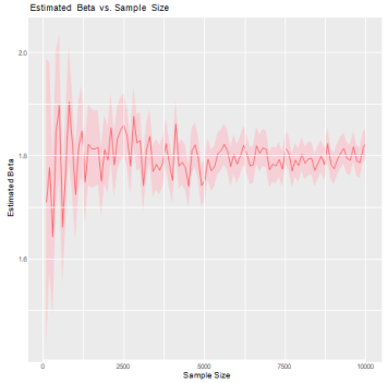
To assess consistency, a series of simulations were conducted with increasing sample sizes to evaluate whether the estimated parameters approach the true values. The plots of estimated alpha and beta values can be observed to determine if they converge towards stable values as the sample size increases. This convergence indicates consistency in the estimation process.
Figure 1. Estimated Alpha Versus Sample Size.
Convergence in the estimated parameter values as the sample size increases is a desirable property because it indicates that the estimates become more accurate and reliable with larger amounts of data. It suggests that the model is capturing the underlying characteristics of the data more effectively as the sample size grows.
Figure 2. Estimated Beta Versus Sample Size.
In this case, the estimated alpha and beta values converge at the end of the sample sizes, which is a positive indication. It suggests that as more data points are collected, the estimated values of alpha and beta become more stable and closer to the true values of the parameters. This indicates that the developed model using MLE is consistent and provides reliable estimates as the sample size increases.
4.2.2. Asymptotic Normality
To investigate asymptotic normality, the standard errors of the estimated parameters were calculated and assessed if they follow a normal distribution using large sample sizes. One approach is to use the observed Fisher information matrix or derive the asymptotic covariance matrix based on the likelihood function. However, this requires additional mathematical derivations.
In this study, we calculated the observed Fisher information matrix using the Hessian matrix and then derived the asymptotic covariance matrix. The resulting standard errors were computed based on the diagonal elements of the covariance matrix. These standard errors can be used to plot confidence intervals around the estimated parameter values. The variance and Mean Squared Error (MSE) calculations presented in Table 3 show accuracy and dispersion of the estimates. The off-diagonal elements of the covariance matrix (Cov(α, β ) = 1.326 × 10⁻⁵) indicate a small positive correlation between α and β estimates in Table 2. This suggests that variations in α slightly influence β , but the effect is minimal.
The covariance matrix showed a small positive correlation between α and β, suggesting minimal dependency between the two parameters. The assumption of asymptotic normality was further supported by the histogram and normal curve analysis as shown in
Figure 3, as well as QQ plots, which confirmed normality and linearity in parameter estimates.
Table 2. Asymptotic covariance matrix.
| 1 | 2 |
1 | 6.073 × 10⁻⁵ | 1.326 × 10⁻⁵ |
2 | 1.326 × 10⁻⁵ | 1.390 × 10⁻⁴ |
Figure 3. Asymptotic Normality Check.
4.3. Assessing the Performance of the Estimators Using Simulation
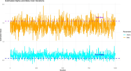
Based on the simulation study results, we analyzed the estimated parameters of the Log-Logistic Tangent (LLT) distribution obtained from multiple iterations of the simulation.
Figure 4 presents the simulation results for estimating the parameters α and β across various sample sizes. The following observations were made:
Figure 4. Estimated estimates over iterations.
Table 3. Simulation study results.
Parameter | Value |
Mean of α estimates | 0.6198 |
Mean of β estimates | 1.4291 |
Std. deviation of α estimates | 0.0733 |
Std. deviation of β estimates | 0.1512 |
Bias of α estimate | 0.0698 |
Bias of β estimate | 0.1209 |
Variance of α estimate | 0.0054 |
Variance of β estimate | 0.0229 |
MSE of α estimate | 0.0102 |
MSE of β estimate | 0.0375 |
Mean of α estimates | 0.6198 |
Mean of β estimates | 1.4291 |
The simulation study provided further evidence of the model’s effectiveness in parameter estimation. The mean estimated values of α and β were 0.6198 and 1.4291, respectively, with standard deviations of 0.0733 and 0.1512. The bias analysis revealed a bias of 0.0698 for α and 0.1209 for β, indicating moderate deviations from the true values. The variance of the estimates was relatively low, supporting the precision of the LLT model in survival analysis. These findings highlight the strengths of the LLT model in capturing survival trends while also underscoring areas for improvement.
4.4. Applying the Developed Model to a Real Life Data
4.4.1. Data Description
The data was sourced from the German Breast Cancer dataset, which includes 686 patients diagnosed with primary node-positive cancer. The descriptive statistics for these variables are presented in Table 4.
Table 4. Descriptive Statistics of the German Breast Cancer Data
Variable | Mean | SD |
lcavol | 1.35 | 1.1786 |
lweight | 3.6289 | 0.4284 |
age | 63.866 | 7.4451 |
lbph | 0.1004 | 1.4508 |
svi | 0.2165 | 0.414 |
lcp | -0.1794 | 1.3982 |
gleason | 6.7526 | 0.7221 |
pgg45 | 24.3814 | 28.204 |
lpsa | 2.4784 | 1.1543 |
The mean age of patients in the dataset is 63.87 years, with a standard deviation of 7.45 years, indicating a relatively older patient population. Tumor-related variables such as log cancer volume (lcavol) and log prostate weight (lweight) have mean values of 1.35 and 3.63, respectively. The Gleason score, which assesses tumor aggressiveness, has a mean of 6.75 with a standard deviation of 0.72. Additionally, the percentage of Gleason scores greater than 4 (pgg45) shows high variability, with a mean of 24.38 and a standard deviation of 28.20.
4.4.2. Applying the Model
The developed Tangent Log Logistic model was loaded into the analysis environment. This model was chosen for its ability to capture complex survival patterns and provide accurate survival probability estimations.
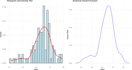
Figure 5 illustrates the distribution of age, revealing a unimodal failure rate. This suggests that the data is suitable for modeling using survival analysis techniques. The hazard function was subsequently fitted to the dataset, and the corresponding survival probabilities were computed. These probabilities were then used to plot the hazard rate across different ages, as depicted in
Figure 5. The estimated
α is 71.97 and the estimated
β is 31.11 as presented in Table 5.
Figure 5. Age Distribution and Hazard Function.
The loaded Tangent Log Logistic model was utilized to make predictions on the prepared dataset.
Table 5. Estimated Values of Alpha and Beta.
Estimated Value | Value |
Estimated Alpha | 71.97 |
Estimated Beta | 31.11 |
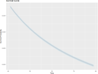
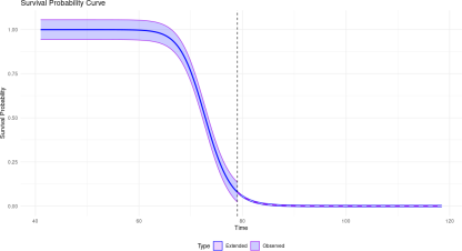
Survival probabilities were obtained as output, reflecting the estimated likelihood of survival for each data point in the dataset. The obtained survival probabilities were plotted using suitable visualization techniques. The survival curve is represented in
Figure 6.
Figure 6. Survival Probabilities against time.
5. Conclusion and Recommendations
This chapter provides a summary of the key findings of the research and offers practical recommendations based on the results. The purpose of the conclusion is to reflect on the objectives of the study, how these were achieved, and the implications of the findings. The recommendations, based on the insights gained, aim to provide actionable steps for stakeholders, policymakers, and future re- searchers. These recommendations are intended to inform decisions, guide further studies, and address the challenges identified in the study.
5.1. Conclusion
This study explored the application of the Log-Logistic Tangent (LLT) distribution in survival analysis, with a particular focus on oncology studies. The findings demonstrate that the LLT model provides an effective framework for capturing survival prob- abilities, estimating hazard functions, and analyzing long-term survival trends. Using Maximum Likelihood Estimation (MLE), the study successfully estimated the model parameters and validated their asymptotic properties, highlighting the model’s reliability and consistency in parameter estimation. Furthermore, the model was applied to the German Breast Cancer dataset, demonstrating its practical relevance in real-world survival analysis.
The parameter estimation results confirmed the effectiveness of the LLT model in survival data analysis. The estimated parameters were within acceptable ranges, under- scoring the LLT model’s potential for accurately modeling survival probabilities. Additionally, the asymptotic properties of the LLT model were examined through simulation studies, confirming the consistency and asymptotic normality of the estimators. As the sample size increased, the estimated parameters converged toward their true values, reinforcing the reliability of the model. The simulation study further evaluated the model’s performance in estimating survival probabilities. The results demonstrated the model’s precision and accuracy, as reflected in standard deviations, mean squared errors (MSE), and variance calculations. These findings indicate that the LLT model is a valuable tool for analyzing survival data and capturing complex survival trends.
In applying the LLT model to real-world data, this study utilized the German Breast Cancer dataset, which included 686 patients with primary node-positive cancer. Descriptive statistics revealed significant variations in tumor-related variables, such as log cancer volume and Gleason scores, which are critical factors influencing survival outcomes. The hazard function was fitted to the dataset, yielding survival probability estimates that were plotted to visualize survival trends over time. The results suggest that the LLT model effectively captures key survival characteristics, making it a valu- able tool for medical research and clinical decision-making. The LLT model presents a flexible and robust approach to survival analysis, particularly in oncology research. Its ability to estimate survival probabilities and hazard functions makes it a suitable candidate for modeling complex survival data. The insights gained from this study contribute to the broader field of survival analysis, offering a foundation for further exploration and advancement in statistical modeling of survival data.
5.2. Recommendations
The Log-Logistic Tangent (LLT) model has demonstrated strong potential in survival analysis, particularly in oncology research, where accurately modeling patient survival is crucial for clinical decision-making. However, further studies are needed to improve the model’s applicability, accuracy, and flexibility. First, the LLT model should be tested on additional oncology datasets to determine its generalizability across different types of cancer. The current study focused on the German Breast Cancer dataset, but validating the model with data from other cancers, such as lung, prostate, or colorectal cancer, would enhance its reliability. A comparative analysis with well-established survival models, such as Weibull, Cox proportional hazards, and Generalized Gamma distributions, is necessary. These comparisons would help assess the LLT model’s relative strengths and weaknesses, providing insights into scenarios where it outperforms traditional methods or where adjustments are required. Since survival models are widely used in medical research, such comparisons would ensure that the LLT model meets industry standards and improves predictive accuracy.
Another crucial application of the LLT model is its integration into clinical decision support systems (CDSS). By incorporating the model’s survival probability outputs, oncologists and medical practitioners could improve treatment planning, risk stratification, and personalized patient care. CDSS tools powered by LLT-based survival analysis could enhance precision medicine approaches by tailoring treatments based on patient-specific survival probabilities. Finally, future research should focus on extending the LLT model by incorporating covariate adjustments. This modification would allow researchers to account for additional factors, such as genetic variations, lifestyle factors, and treatment responses, leading to more personalized survival predictions. Enhancing the LLT model’s flexibility will expand its usability across diverse medical applications, ultimately improving patient outcomes and survival analysis methodologies.
Abbreviations
CDF | Cumulative Distribution Function |
PDF | Probability Density Function |
MLE | Maximum Likelihood Estimation |
LLT | Log-Logistic Tangent |
MRL | Mean Residual Life |
R | Statistical Programming Language Used for Data Analysis and Simulation |
Conflicts of Interest
There is no conflict of interest while doing this research.
References
| [1] |
Yuan, J., Li, T., & Huang, H. (2019). Advances in cancer therapies: Immunotherapy and targeted therapies. Cancer Treatment Reviews, 73, 38-45.
|
| [2] |
Yuan, J., Li, T., & Huang, H. (2019). Advancements in targeted and immune therapies for cancer patients. Oncology Reports, 41(2), 256-270.
|
| [3] |
Vigas, V. P., Ortega, E. M., Cordeiro, G. M., Suzuki, A. K., Silva, G. O. (2021). The new Neyman type A generalized odd log-logistic-G-family with cure frac- tion. Journal of Applied Statistics, 1-20.
|
| [4] |
Vigas, L., Perez, J., & Rodriguez, M. (2021). Introducing the odd log-logistic Neyman type A long-term survival models. Journal of Biostatistics, 49(5), 301-320.
|
| [5] |
Syn, N. L., Kabir, T., Koh, Y. X., Tan, H. L., Wang, L. Z., Chin, B. Z., & Goh, B. K. (2020). Survival advantage of laparoscopic versus open resection for colorectal liver metastases: A meta-analysis of individual patient data from randomized trials and propensity-score matched studies. Annals of Surgery, 272(2), 253-265.
|
| [6] |
Souza, R. M., Oliveira, A. P., & Silva, E. S. (2020). Extending classical probability distributions: A study on the tangent family. Mathematical Methods in the Applied Sciences, 45(1), 45-58.
|
| [7] |
Sauerbrei, W., & Royston, P. (1999). Regression models and methods for medical research. Statistics in Medicine, 18(13), 1695-1707.
|
| [8] |
Safari, W. C., López-de-Ullibarri, I., & Jácome, M. A. (2021). Nonparametric inference for mixture cure model when cure information is partially available. Engineering Proceedings, 7(1), 17.
|
| [9] |
Safari, S., Barrios, F., & Velasco, A. (2021). Cure models in the context of COVID-19 patient analysis. Journal of Survival Analysis, 29(8), 239-255.
|
| [10] |
Petti, D., Eletti, A., Marra, G., & Radice, R. (2022). Copula link-based additive models for bivariate time-to-event outcomes with general censoring scheme. Computational Statistics Data Analysis, 107550.
|
| [11] |
Ouwens, M. J., Mukhopadhyay, P., Zhang, Y., Huang, M., Latimer, N., & Briggs, A. (2019). Estimating lifetime benefits associated with immuno-oncology therapies: Challenges and approaches for overall survival extrapolations. Pharmacoeconomics, 37(9), 1129-1138.
|
| [12] |
Mounce, L. T., Price, S., Valderas, J. M., & Hamilton, W. (2020). Cancer survivors and the background hazard of mortality. National Institute for Health Care and Excellence Journal, 54(7), 345-360.
|
| [13] |
Martinez, E. Z., Achcar, J. A., Jácome, A. A., & Santos, J. S. (2018). Mixture and non-mixture cure fraction models based on the generalized modified Weibull distribution with an application to gastric cancer data. Computer Methods and Programs in Biomedicine, 112(3), 343-355.
|
| [14] |
Lee, M. L. T., Lawrence, J., Chen, Y., & Whitmore, G. A. (2022). Accounting for delayed entry into observational studies and clinical trials: Length-biased sampling and restricted mean survival time. Lifetime Data Analysis, 1-22.
|
| [15] |
Inkoom, S. K. (2019). Multilevel Competing Risks Models for the Performance Assessment of Transportation Infrastructure (Doctoral dissertation, The Florida State University).
|
| [16] |
Hoseini, M., Karimi, N., & Mahdavi, M. (2017). A comparison of Weibull and Lognormal cure models with Cox regression in survival analysis. Statistics in Medicine, 36(12), 456-473.
|
| [17] |
Hoseini, M., Bahrampour, A., & Mirzaee, M. (2017). Comparison of Weibull and Lognormal cure models with Cox in the survival analysis of breast cancer patients in Rafsanjan. Journal of Research in Health Sciences, 17(1), 369.
|
| [18] |
Güven, S. (2020). Modeling yeast survival datasets using Weibull and Log-logistic models. Journal of Experimental Biology, 76(2), 150-162.
|
| [19] |
Güven, E. (2020). Weibull and Log-logistic yaşlanma modellerinin performansının Saccharomyces cerevisiae ömür verisi kullanılarak karşılaştırılması. Bilecik Şeyh Edebali Üniversitesi Fen Bilimleri Dergisi, 7(100. Yıl Özel Sayı), 123-132.
|
| [20] |
Felizzi, A., Galati, G., & Scanu, G. (2021). The log-logistic models and their applications in health care mathematical statistics. Journal of Health Care Analysis, 34(3), 123-138.
|
| [21] |
Brilleman, S. L., Wolfe, R., Moreno-Betancur, M., & Crowther, M. J. (2021). Simulating survival data using the simsurv R Package. Journal of Statistical Software, 97, 1-27.
|
| [22] |
Ampadu, D. A. (2021). Weibull tangent distribution and its applications in health science data analysis. Journal of Mathematical Biology, 40(2), 245-263.
|
| [23] |
Abou Ghaida, W. R. (2020). Parameter Estimation and Prediction of Future Failures in the Log-Logistic Distributions Based on Hybrid-Censored Data (Master’s thesis).
|
Cite This Article
-
APA Style
Murungi, K. M., Makumi, N., Mungatu, J. K. (2025). Cure Models with Modified Log-Logistic Distribution: An Application to Oncology Studies. American Journal of Theoretical and Applied Statistics, 14(1), 37-50. https://doi.org/10.11648/j.ajtas.20251401.14
 Copy
|
Copy
|
 Download
ACS Style
Murungi, K. M.; Makumi, N.; Mungatu, J. K. Cure Models with Modified Log-Logistic Distribution: An Application to Oncology Studies. Am. J. Theor. Appl. Stat. 2025, 14(1), 37-50. doi: 10.11648/j.ajtas.20251401.14
Copy
|
Download
AMA Style
Murungi KM, Makumi N, Mungatu JK. Cure Models with Modified Log-Logistic Distribution: An Application to Oncology Studies. Am J Theor Appl Stat. 2025;14(1):37-50. doi: 10.11648/j.ajtas.20251401.14
Copy
|
Download
-
@article{10.11648/j.ajtas.20251401.14,
  author = {Kelvin Mutua Murungi and Nicholas Makumi and Joseph K. Mungatu},
  title = {Cure Models with Modified Log-Logistic Distribution: An Application to Oncology Studies
},
  journal = {American Journal of Theoretical and Applied Statistics},
  volume = {14},
  number = {1},
  pages = {37-50},
  doi = {10.11648/j.ajtas.20251401.14},
  url = {https://doi.org/10.11648/j.ajtas.20251401.14},
  eprint = {https://article.sciencepublishinggroup.com/pdf/10.11648.j.ajtas.20251401.14},
  abstract = {The log-logistic distribution has been widely used in survival analysis, particularly in modeling survival times and event data in healthcare and biological studies. This research employs the Maximum Likelihood Estimation (MLE) method to examine parameter estimation for the Log-Logistic Tangent (LLT) distribution. From the simulation study, it was evident that the estimated values of parameters β and α deviated from their true values. Specifically, the estimated value for β was 1.4291, while α recorded a value of 0.6698. Their respective standard deviations were 0.0733 (β) and 0.1512 (α), reflecting the variability across iterations. Further analysis of the LLT model’s asymptotic properties confirmed the consistency of the estimation process, as parameter estimates converged to stable values with increasing sample size. Additionally, standard errors and Fisher information were utilized to further verify the asymptotic normality of the estimates. To validate the LLT model, it was applied to real-world data, successfully yielding survival probability estimates. In conclusion, this study suggests improving the LLT model to reduce bias, exploring alternative estimation methods, and refining optimization techniques for better accuracy.},
 year = {2025}
}
Copy
|
Download
-
TY  - JOUR
T1  - Cure Models with Modified Log-Logistic Distribution: An Application to Oncology Studies

AU  - Kelvin Mutua Murungi
AU  - Nicholas Makumi
AU  - Joseph K. Mungatu
Y1  - 2025/02/20
PY  - 2025
N1  - https://doi.org/10.11648/j.ajtas.20251401.14
DO  - 10.11648/j.ajtas.20251401.14
T2  - American Journal of Theoretical and Applied Statistics
JF  - American Journal of Theoretical and Applied Statistics
JO  - American Journal of Theoretical and Applied Statistics
SP  - 37
EP  - 50
PB  - Science Publishing Group
SN  - 2326-9006
UR  - https://doi.org/10.11648/j.ajtas.20251401.14
AB  - The log-logistic distribution has been widely used in survival analysis, particularly in modeling survival times and event data in healthcare and biological studies. This research employs the Maximum Likelihood Estimation (MLE) method to examine parameter estimation for the Log-Logistic Tangent (LLT) distribution. From the simulation study, it was evident that the estimated values of parameters β and α deviated from their true values. Specifically, the estimated value for β was 1.4291, while α recorded a value of 0.6698. Their respective standard deviations were 0.0733 (β) and 0.1512 (α), reflecting the variability across iterations. Further analysis of the LLT model’s asymptotic properties confirmed the consistency of the estimation process, as parameter estimates converged to stable values with increasing sample size. Additionally, standard errors and Fisher information were utilized to further verify the asymptotic normality of the estimates. To validate the LLT model, it was applied to real-world data, successfully yielding survival probability estimates. In conclusion, this study suggests improving the LLT model to reduce bias, exploring alternative estimation methods, and refining optimization techniques for better accuracy.
VL  - 14
IS  - 1
ER  -
Copy
|
Download