Assessing the Quality of Ordinary Least Squares in General L<sup>p</sup> Spaces

Kevin Hoffman; Hugo Moises Montesinos-Yufa

doi:doi:10.11648/j.ajtas.20241306.12

Research Article |

| Peer-Reviewed

Assessing the Quality of Ordinary Least Squares in General L^p Spaces

Kevin Hoffman

, Hugo Moises Montesinos-Yufa^*

Published in American Journal of Theoretical and Applied Statistics (Volume 13, Issue 6)

Received: 20 September 2024 Accepted: 18 October 2024 Published: 18 November 2024

Views: Downloads:

Download PDF

Share This Article

Twitter
Linked In
Facebook

Abstract

In the context of regression analysis, we propose an estimation method capable of producing estimators that are closer to the true parameters than standard estimators when the residuals are non-normally distributed and when outliers are present. We achieve this improvement by minimizing the norm of the errors in general L^p spaces, as opposed to minimizing the norm of the errors in the typical L² space, corresponding to Ordinary Least Squares (OLS). The generalized model proposed here—the Ordinary Least Powers (OLP) model—can implicitly adjust its sensitivity to outliers by changing its parameter p, the exponent of the absolute value of the residuals. Especially for residuals of large magnitude, such as those stemming from outliers or heavy-tailed distributions, different values of p will implicitly exert different relative weights on the corresponding residual observation. We fitted OLS and OLP models on simulated data under varying distributions providing outlying observations and compared the mean squared errors relative to the true parameters. We found that OLP models with smaller p's produce estimators closer to the true parameters when the probability distribution of the error term is exponential or Cauchy, and larger p's produce closer estimators to the true parameters when the error terms are distributed uniformly.

Published in	American Journal of Theoretical and Applied Statistics (Volume 13, Issue 6)
DOI	10.11648/j.ajtas.20241306.12
Page(s)	193-202
Creative Commons	This is an Open Access article, distributed under the terms of the Creative Commons Attribution 4.0 International License (http://creativecommons.org/licenses/by/4.0/), which permits unrestricted use, distribution and reproduction in any medium or format, provided the original work is properly cited.
Copyright	Copyright © The Author(s), 2024. Published by Science Publishing Group

Keywords

Regression Analysis, Least Squares, Robust Regression, Outliers, Simulation

1. Introduction

Ordinary Least Squares (OLS) regression is a benchmark technique that is used for its computational ease-of-use and its calculation of the best, linear, unbiased, and efficient (BLUE) estimators when the classical normal linear regression model (CNLRM) assumptions are met. Coefficients are estimated by minimizing the sum of squared residuals. As a result, residuals have a disproportional (squared) influence over the estimators. The estimators, thus, are especially sensitive to large residuals.

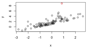
A large sensitivity could be problematic because outlying residuals can have an overwhelming influence on the accuracy of the model’s coefficients. The estimators tend to deviate further from the true parameters when there are more outliers in the data. Different sensitivities of the estimators to the residuals could be more appropriate depending on how the residuals are distributed and the probability of observing outliers. For example, outlying residuals are more likely when the underlying probability distribution of the error term is exponential, or a mixture of exponentials and normals, than when it is purely normal. The occurrence of outlying residuals can deviate the estimation away from the true parameters, especially if large residuals are given large weights. In Figure 1, the red point (

y \geq 8

) is an outlier. If one were to decrease the sensitivity of the estimators to the residuals, then the red point (

y \geq 8

) would have less influence over the estimators. Changing this sensitivity could produce estimators closer to the true parameters.

Download: Download full-size image

Figure 1. Scatterplot of two positively correlated variables (x and y) simulated in such a way that the error term follows an exponential probability distribution. Note the tendency towards positive residuals. The largest residual (

y \geq 8

) is shown in red.

1.1. Robust Methods

In the presence of outliers, robust regression techniques can produce better estimators than standard OLS or even maximum likelihood (ML) estimators. Essentially, the idea of robust methods is to give less ‘weight’ to potential outlying observations. In cases of large residuals, robust methods results may vary significantly from OLS’s

[1-6]

. In cases where robust methods produce significantly different estimators than their non-robust counterparts, the differences may be due to outlying observations stemming from either fat tails or an asymmetric probability distribution of the underlying error term. In both cases, extreme observations can deviate the estimation results significantly, and erratically, from the true parameters, creating the need for methods that are less sensitive, or more robust, to these observations. In essence, the sensitivity to extreme observations is at the heart of robust methods and plays a significant role in our analysis.

One common example of a robust method is quantile regression. Quantile regression operates using the median (and more generally, any quantile) instead of the average as a point estimator

[1-3, 7-9]

. While this is effective at reducing the influence of outlying observations, it is limited to the L¹ space. Instead of limiting itself to the L² space (OLS regression) or the L¹ space (Quantile Regression), we conjecture that a more general model could exist in more general L^p spaces. Like quantile regression in the L¹ space, the use of general L^p spaces could achieve the goal of reducing the regression sensitivity to outliers in a more flexible way. Notably, this model would regulate sensitivity as a function of its residing space.

[10, 11]

There have been a few attempts to model regression in L^p spaces. For example, some scholars have moved away from OLS to analyze 3D scanning datasets containing outliers and missing data

[12]

. By experimenting with alternative exponents in the cost function of the residuals, they were essentially exploring alternative L^p spaces on their results. In summary, they found better and more sensible results in their specific applications using

p \neq 2

. That is, when modeling in L^p spaces with p’s different from two, their scans would approximate their original image best

[12]

. These findings are crucial for motivating our research questions. Are these 3D scanning results specific to this application or is there a more general pattern of potential improvement over standard regression methods? If so, under which conditions could improvement be achieved? Our study is a first step in this direction. We systematically analyze the usage of regression in L^p spaces under different probabilistic distributional assumptions for the error term. This is the central goal of this paper.

2. Methods

In this section, we propose a general method for regression analysis in L^p spaces. We call this method Ordinary Least Power (OLP) and briefly present the math behind it vis-à-vis the math behind the Ordinary Least Squares (OLS) method. In a general L^p space (OLP method), our goal would be to minimize the sum of the absolute value of the residuals to the ‘p’th power (

\min \sum_{i = 1}^{n} {|e_{i}|}^{p}

), whereas in L² (OLS) the goal is to minimize the sum of the residuals the squared power (

\min \sum_{i = 1}^{n} e_{i}^{2}

). See Table 1 for the equations corresponding to the first-order condition for optimization.

Table 1. First Order Optimality Conditions for OLS and OLP

(p \neq 1)

corresponding to Population Model

y_{i} = β_{0} + β_{1} * x_{i} + ϵ_{i}

Ordinary Least Squares (OLS) Normal Equations

Ordinary Least Power (OLP) “Normal” Equations, given p.

$\frac{\partial F}{\partial {\hat{β}}_{0}} = - 2 * (y_{i} - {\hat{β}}_{0} - {\hat{β}}_{1} * x_{i})^{2 - 1} = 0$

$\frac{\partial F}{\partial {\hat{β}}_{1}} = 2 * (y_{i} - {\hat{β}}_{0} - {\hat{β}}_{1} * x_{i})^{2 - 1} * - x_{i} = 0$

$\frac{\partial F}{\partial {\tilde{β}}_{0}} = - p * | y_{i} - {\tilde{β}}_{0} - {\tilde{β}}_{1} * x_{i} |^{p - 1} = 0$

$\frac{\partial F}{\partial {\tilde{β}}_{1}} = p * | y_{i} - {\tilde{β}}_{0} - {\tilde{β}}_{1} * x_{i} |^{p - 1} * - x_{i} = 0$

The fundamental difference lies in the residual’s exponent. The residual in the OLS model is

e_{i}^{OLS} = (y_{i} - {\hat{β}}_{0} - {\hat{β}}_{1} * x_{i})

. The residual in the OLP model is

e_{i}^{OLP} = (y_{i} - {\tilde{β}}_{0} - {\tilde{β}}_{1} * x_{i})

. The optimal solutions of these two models are not equal unless

p = 2

, in which case the results of OLS and OLP are identical, by construction. That is, if

p = 2,

then

the intercepts are equal (

{\hat{β}}_{0} \equiv {\hat{β}}_{0, OLS} = {\tilde{β}}_{0} \equiv {\hat{β}}_{0, OLP})

and the slopes are also equal (

{\hat{β}}_{1} \equiv {\hat{β}}_{1, OLS} = {\tilde{β}}_{1} \equiv {\hat{β}}_{1, OLP})

In general, the OLP estimators cannot be obtained directly or in closed form as their OLS counterparts. This is because the key equations to solve, the first-order conditions for optimization shown above, are not “normal” or “orthogonal” anymore because they are derived from functions outside the L2 space. We therefore used Newton-Rapson numerical optimization methods to solve for the OLP estimates. Newton’s method takes initial root guesses on the parameters (slope and intercept), calculates the error, and iterates until a solution is achieved

[13, 14]

. It makes sequential root guesses based on the information from previous iterations until the roots converge to the final solutions (provided a solution exists). When p equals two, we confirmed numerically that our OLP implementation matches the OLS solution and that slight deviations away from

p = 2

produced estimators slightly away from those of the OLS method.

The first step in analyzing the qualities of the OLP method is to determine if the OLP estimators are significantly different from the OLS estimators. We ran statistical tests of difference in means for the difference between the mean squared error (MSE) of the OLP estimators and the OLS estimators. Our MSE is calculated with respect to the true parameters in our simulation. For simulation purposes, we set the true slope and intercept equal to 1 in our data generating process. We simulated the data using error terms following the normal, uniform, exponential (asymmetric), and Cauchy probability distributions. In our baseline simulation, we used a sample size of n = 1,000 observations. We then calculated the MSEs of the OLS estimators and the MSEs of the OLP estimators, both with respect to the true simulated parameters. We did this for p’s ranging from 1.2 to 2.8 in increments of 0.1 and we repeated these steps 2,000 times. We ran both standard t-tests and non-parametric versions of the difference in means tests for the two MSEs. In both cases, the p-values of the tests were low for certain values of the parameter p of OLP, indicating that the OLS and OLP estimators are significantly different in certain applications or under certain conditions. We report the results of the t-tests in Figures 2 and 3 and elaborate on these differences further below.

The next step in analyzing the OLP method is to determine if the difference in OLS and OLP estimators is beneficial or detrimental in terms of their mean squared error. We compared the t-statistics to the p’s of the OLP method over the four different error term probability distributions. The t-test measured the difference in MSEs (MSE_OLS-MSE_OLP). Defined this way, a positive sign indicates that the OLP method has a lower (better) MSE than the OLS counterpart, and a negative sign indicates the opposite. Therefore, if the OLP method yields estimators systematically closer to the true parameter than the OLS method, then we would expect positive values for the t-tests. More importantly, we are interested in the relationship between the sign and magnitude of the t-statistic and the different values of the parameter p of the OLP method. We are also interested in learning how this relationship would change with different probability distributions of the error term.

We also took a simulation approach to examine the asymptotic properties of our OLP method. To that end, we explored if the mean square error of the OLP estimators approaches to zero as the sample size increases (that is, to assess asymptotic consistency). Convergence in mean square error guarantees (i.e., is a sufficient condition) for convergence in probability, which is what we need for consistency. Therefore, we specifically proceeded as follows: We generated datasets with varying sample sizes (n = 10, 50, 100, 500, and 1000) for each error term probability distribution (normal, exponential, uniform, and Cauchy). We repeated the process 500 times for each sample size and probability distribution combination. We then evaluated the linear relationship between the MSE of the OLP model and the samples sizes of the simulation using a standard OLS regression model. Technically, we first employed a double logarithmic transformation to “linearize” the data and then estimate the linear relationship of the transformed data (or equivalently, an exponential relationship of the original data). Another technical issue is that because the varying sample sizes (n) imply a varying precision in the OLP estimation, there is an induced (and inevitable) heteroskedasticity in our MSE_OLP making it more precise for large sample sizes and more volatile for small sample sizes. This heteroskedasticity may need to be corrected by weighting the OLS regression by the sample size. Therefore, to assess consistency using simulation, we examined the relationship between the MSE_OLP and the sample size before and after correcting for heteroscedasticity.

3. Results

We first compared if the mean squared errors (MSEs) of the OLS method were significantly different from the MSEs of the OLP method. Statistically, we focused on both the p-value and t-statistic associated with this difference. We first analyzed the p-value and found that it became increasingly significant (smaller in value), on average, as the parameter p of the OLP method deviated from two (Figure 2). This meant that the MSEs of OLS and OLP estimators became more and more statistically different from each other as p’s distance from two increases. This would only tell us that one method is significantly better than the other, but nothing more. Our following task would be, of course, to investigate which method is better; and more importantly, under which conditions one method is better than the other, and vice versa. One of such important conditions to investigate is the probability distribution of the error term.

Download: Download full-size image

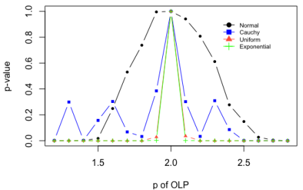
Figure 2. The OLP and OLS methods for different values of the parameter p of OLP. This figure shows the statistical significance (p-value) from a t-test of the difference in means between the MSE from the OLS method and the MSE from the OLP method for different values of the parameter p of OLP ranging from 1.2 to 2.8 in 0.1 increments. All MSEs are calculated with respect to the true parameters in the simulation using four probability distributions for the error terms. The black dots come from normally distributed error terms, the blue squares come from Cauchy distributed error terms, the green crosses come from asymmetrically (exponentially) distributed error terms, and the red triangles come from the uniformly distributed error terms. The sample size was n=1,000 observations and we employ 2,000 replications for each level of p of OLP and for each probability distribution.

When the error term was non-normally distributed, changing the parameter p of the OLP method had a larger influence on the difference in MSEs between the OLP and OLS methods, than when the error term was normally distributed. Specifically, using error terms following the uniform, exponential (asymmetric), and Cauchy probability distributions, the p-value of the difference in MSEs converged to zero rapidly as the parameter p of OLP deviated away from two. This was the first indication that one of the key conditions under which the methods OLP and OLS deviate significantly from each other, is precisely the probability distribution of the error term. This makes intuitive sense because, in our setting, the distribution of the error term is the only law that governs, probabilistically, the size and frequency of outliers in our data.

In addition to the normal, our benchmark distribution, we wanted to use the uniform, exponential, and Cauchy distribution for different reasons. The exponential distribution brings asymmetric errors, inducing a systematic bias in the intercept. The Cauchy distribution is of especial interest because of its extremely fat tails given the fact that its moments, especially its mean and variance, do not exist. Also, due to its very fat tails, outliers occur with high probability (and therefore very frequently). Thus, the Cauchy distribution is a natural candidate to provide a systematic source of large and frequent outlying observations. Finally, the uniform distribution leads to the exact opposite rationale. Because all observations are confined withing the lower and upper bound parameters, there are no possible outliers coming from this distribution. This intuition is consistent with the uniform being the distribution with the maximum entropy among the class of all continuous distributions in a connected interval.

As shown in Figure 2, when

p = 2

(or when

p ≅ 2

) the methods OLS and OLP are indistinguishable regardless of the probability law of the error term. But when

p

deviates significantly from 2, the p-values of the difference in means test converge to zero almost monotonically with the function

|p - 2|

, except for the Cauchy probability distribution. Given the nature of the Cauchy distribution, it is expected that the convergence of the p-values to zero was not perfectly monotonic in our simulations. This result reflects the presence of large outliers in some of our simulated error terms when using the Cauchy probability distribution (see Figure 2, blue squares).

As mentioned above, while low p-values tell us that there is a significant difference between OLP and OLS estimators, the sign of the test statistic tells us the direction of the difference, i.e., which one is better in terms of mean squared error. Given that the t-statistics were based on the difference of MSE_OLSminus MSE_OLP, a positive sign would indicate that the OLP estimator is better (lower MSE for the OLP method). If the sign is negative, then the OLS estimator is deemed superior.

As shown in Figure 3, when the error term was normally distributed (black dots), the t-statistic was clearly negative for p’s far away from two and around zero for p’s close to two. This indicated that the OLP estimators were worse than the OLS estimators when the residuals were normally distributed. This was true for all values of p of OLP, excluding p equals two. Overall, when the error term is normally distributed, OLP converges to OLS when p approaches two. This result is reassuring given the optimal properties of OLS estimators under normally distributed errors. As expected, OLP diverges away from OLS when p differs from two.

Download: Download full-size image

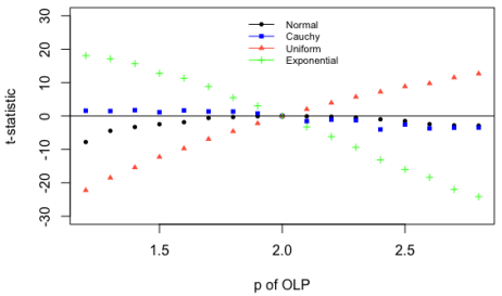
Figure 3. The OLP and OLS methods for different values of the parameter p of OLP. This figure shows the statistical significance (t-value) from a t-test of the difference in means between the MSE from the OLS method and the MSE from the OLP method for different values of the parameter p of OLP ranging from 1.2 to 2.8 in 0.1 increments. Given that the t-statistic was based on MSE_OLS - MSE_OLP, a positive sign would indicate that the OLP estimator is better (lower MSE for the OLP method). All MSEs are calculated with respect to the true parameters in the simulation using four probability distributions for the error terms. The black dots come from normally distributed error terms, the blue squares come from Cauchy distributed error terms, the green crosses come from asymmetrically (exponentially) distributed error terms, and the red triangles come from the uniformly distributed error terms. The sample size was n=1,000 observations and we employ 2,000 replications for each level of p of OLP and for each probability distribution.

When the error term was exponentially distributed (green crosses in Figure 3), the t-statistic was positive for p’s less than two, around zero for p’s close to two, and negative for p’s greater than two. This meant that the OLP method was better than the OLS method when p was less than two and the OLS method was better when p was larger than 2. When the parameter p of OLP equaled two, then OLS and OLP produced the same results. Generally, there is evidence that OLP’s estimators became increasingly better as p decreased given the exponential probability distribution of the error term (Figure 3).

An opposite result was observed when the error term had a uniform probability distribution (red tringles in Figure 3). The t-statistic was negative for p’s less than two, around zero for p’s close to two, and positive for p’s greater than two. This meant that OLS was better than OLP when p was less than two, they were equivalent when p equaled two, and OLP was better than OLS when p was greater than two. There was a clear positive relationship between the parameter p of OLP and the t-statistic when the error term followed a uniform probability distribution (Figure 3, red triangles). The opposite/mirroring results between the uniform and exponential error terms were remarkable. This finding suggest that a lower p is best suited for error term probability distributions with frequent outliers (such as the exponential), while a larger p is best suited for probability distributions with infrequent outliers (such as the uniform).

We also explored the Cauchy probability distribution given its undefined probability moments and fat tails. When the probability distribution of the error term was Cauchy, the OLP method was slightly better than the OLS method when p was less than two, the two methods were equivalent when p was close to two, and the OLS method was slightly better than the OLP method when p was larger than two (Figure 3, blue squares). Unlike the other probability distributions (exponential, uniform, and normal), when the error term was distributed Cauchy, the magnitude of the t-statistic was relatively small and less sensitive to changes in p.

Download: Download full-size image

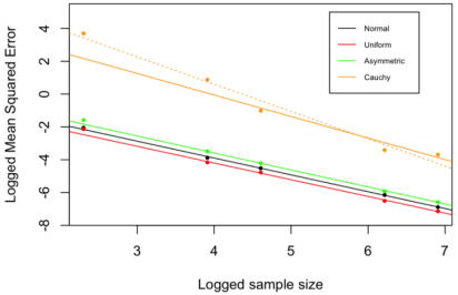
Figure 4. The natural logarithm of the mean squared error (MSE) and the natural logarithm of the sample size for four different probability distributions of the error term: Normal, Uniform, Exponential (Asymmetric), and Cauchy. The variables were logged to allow for a more linear relationship. Due to heteroskedasticity, weighted least squares (WLS) was implemented using the samples size as weights. The heteroskedasticity correction mattered only for the Cauchy probability distribution but not the other distributions (the other dash and solid lines overlap). The dashed line represents the pre-weighted regression model. Each point represents an average after 500 simulations. Sample sizes were 10, 50, 100, 500, and 1000. The MSE is the mean squared error of the OLP estimators with respect to the true simulated parameters.

Our understanding of the OLP method would be enhanced by exploring its asymptotic statistical properties, such as consistency. As mentioned above, a sufficient condition for consistency is that the MSE converges to zero as the sample size increases. We examined the asymptotic consistency of the OLP method by analyzing the relationship between its MSE and the sample size. For all probability distributions of the error term tested here, the natural logarithm of the mean squared error from the OLP model decreased linearly as the natural logarithm of the sample size increased (Figure 4). This finding indicates that the OLP estimators become closer to the true parameters as the sample size increases, which is a desirable characteristic reflecting the asymptotic consistency of the OLP method.

Table 2. The rate of asymptotic convergence of the OLP method as estimated by weighted least squared (WLS) of the log MSE on log sample size using four probability distribution: Cauchy (column 1), normal (column 2), uniform (column 3), and exponential/asymmetric (column 4). Each column represents the probability distribution of the error term when estimating an OLP model using different sample sizes (n = 10, 50, 100, 500, and 1000). Standard errors are in parentheses

[15]

	Mean Squared Error
	Cauchy	Normal	Uniform	Exponential (Asymmetric)
	(1)	(2)	(3)	(4)
Sample Size	-1.313**	-1.027***	-1.019***	-1.035***
Sample Size	(0.246)	(0.014)	(0.031)	(0.022)
Constant	5.196** (1.595)	0.210* (0.089)	-0.127 (0.204)	0.551** (0.143)
R²	0.905	0.999	0.997	0.999
Adjusted R²	0.873	0.999	0.996	0.998
Residual Std. Error (df=3)	8.041	0.447	1.030	0.723
F Statistic (df = 1; 3)	28.6	5,654.8	1,047.2	2,198.0

Notes:*p<0.1; **p<0.05; ***p<0.01

The slope of the regression models in Table 2 shed light on the speed of convergence. For OLP models with the Cauchy, normal, uniform, and asymmetric (exponential) probability distributions of the error term, we chose OLP methods with the following parameter p: Cauchy distribution, p equal 1.5; Normal distribution, p equal 2; Uniform distribution, p equal 2.5; and Exponential distribution, p equal 1.5. We chose these parameters because they are in the optimal/beneficial range (the t-statistic is positive) for the usage of OLP under each probability distribution, as shown in Figure 3. The results using these four probability distributions are presented in columns one, two, three, and four of Table 2, respectively. In all cases, (columns one to four), the estimated slope coefficient was not statistically different from

- 1

. This indicates that the MSE of the OLP method converges to zero at the rate proportional to

n^{- 1}

. See Proposition 1, below.

Proposition 1: If the Mean Square Error and the sample size are related according to a power law, then we can use linear regression analysis to investigate this relationship:

\log (MSE) = a + b * \log (n) .

Moreover, the MSE would be inversely proportional to the sample size if b, the slope in the log-log regression model is equal to minus one

(b = - 1)

Proof:

We start with the log-log linear relationship between the mean square error (MSE) and the sample size

n

\log (MSE) = a + b \log (n) .

Taking

\exp (∙)

on both sides, we get

MSE = \exp (a + b \log (n)) .

Which, after some algebra, becomes

MSE = \exp (a) \exp (b \log (n))

MSE = \exp (a) \exp (\log (n^{b}))

MSE = \exp (a) n^{b}

MSE = a^{'} n^{b}

Where

a^{'} \equiv \exp (a)

is the exponential of the intercept term estimated in Table 2, and

b

is the slope term also estimated in Table 2. Therefore, if

b = - 1

, our findings would indicate that the MSE is inversely proportional to the sample size (that is,

MSE \propto n^{- 1})

. We can directly test this result statistically by conducting the following hypothesis test:

H 0 : b = - 1 versus H 1 : b \neq - 1

Indeed, this is precisely what Table 2 accomplishes. In the simulations performed, all coefficient estimates are within 2 standard errors of the unitary slope, yet the critical t-value for 95% confidence and 3 degrees of freedom is 3.18 (standard errors). This indicates that we can’t reject H0 in any of the simulations performed in Table 2. Therefore, under the null hypothesis of

b = - 1

, we get:

MSE = a^{'} n^{- 1} = \frac{a^{'}}{n}

Or, put more simply:

MSE \propto n^{- 1}

The regression results in Table 2 also showed very high r-squares, being over 0.99 for the normal (column 2), exponential (column 3) and uniform (column 4) probability distributions and being above 0.9 in the case of the Cauchy probability distribution (column 1). This indicates that almost all the variation in the observed MSE can be explained by the sample size for each of the error term probability distributions in Table 2. Given that these are average MSEs over 500 replications; one average for each of the five sample sizes (n = 10, 50, 100, 500, and 1000), the high r-squares are not surprising. When the error term followed a Cauchy probability distribution, a lower r-squared is also expected because of the higher variation in mean squared error in the data would translate into more volatile OLP results when compared to the other probability distributions of the error term.

4. Discussion

The performance of the usual regression methods (and the OLS method in particular) is substantially hindered by the presence of outliers. This is because the OLS estimators operate in the L² space and are therefore especially influenced, in a squared manner, by large residuals. Some robust regression methods have partially addressed the estimators’ sensitivity to outliers but they still remain confined to a single space, typically either the L¹ or the L² spaces

[3, 5, 9, 14]

. The goal of our paper was to improve upon the standard regression techniques in the presence of outliers by allowing the estimation of regression parameters in more general L^p spaces and examining the properties of the proposed estimators, the Ordinary Least Power (OLP) estimators, under different probability distributions of the error term. We tested the OLP method vis-à-vis the OLS method by comparing their MSEs and analyzing their asymptotic properties. In theory, the OLP method could adapt to varying probability distributions of data by selecting a beneficial parameter p that would yield lower MSEs and therefore estimators closer to the true parameters.

Using simulation, we determined that the OLP and OLS methods are significantly different when the p of OLP deviates significantly from two. The amount that p had to differ from two depends on the presence of outliers in our data. We used the normal, exponential, Cauchy, and uniform probability distributions of the error term to control the size, frequency, and direction of the outliers. In general, when the error term was non-normally distributed, a deviation of the parameter p of OLP away from two, resulted in a more distinguishable difference between the OLS and OLP methods (as measured by the p-value of the difference in their average MSEs). This indicates that changing p has a more impactful influence on the estimators when the error term is non-normally distributed.

Looking at difference in mean square errors between the OLP and OLS methods, we found that when the error term was normally distributed, the OLS method was always better or the same as (but never worse than) the OLP method. This result was expected and reassuring because the OLS method is designed to perform well with normal error terms. Setting the parameter p of the OLP method equal to two (which is essentially the same as an OLS model) is therefore the natural optimal choice with normally distributed data.

In turn, with asymmetric (exponential) and Cauchy probability distributions of the error term, there was a larger presence of outliers. As a result, a parameter p of OLP less than two provided better estimators than OLS’s. Selecting a small p could be beneficial in a situation of outliers because it gives less implicit weight to large residual observations. Therefore, when the error term was distributed in such a way that permitted more frequent and larger outliers (exponentially or Cauchy), setting the parameter p of OLP lower than two improved the accuracy and precision of the OLP estimators relative to the OLS estimators. There was a noticeably better effect of lowering p when the error term was asymmetrically (exponentially) distributed than Cauchy which could be since the Cauchy distribution has no defined mean or variance.

The opposite result was observed when the error term was uniformly distributed. A larger p provided better estimators than OLS’s. Intuitively, raising the parameter p of OLP should give a greater influence to large residuals, and lowering p decreases the influence of large residuals. The uniform probability distribution has no outliers by definition. Therefore, it seems that raising p beyond two allows the model to take into full account small patterns in the data that would be undermined by a lower p while exploiting the flexibility of the general L^p spaces. Selecting a parameter p of OLP greater than two could be beneficial for bounded datasets with large entropy and containing fewer (and less frequent) outliers than would be expected under normal data.

Measuring the asymptotic properties (the consistency, in particular), of the OLP method via simulation was important for two main reasons. First, it is useful to observe a consistent reduction in the bias, variance, and MSE with larger sample sizes because it allows for increased confidence in the predictions and analysis. Second, it highlights the similarity between the OLP and OLS methods rather than their differences. This is important to improve upon OLS limitations in future research while maintaining its advantages. Confirming that OLP estimators are consistent is an essential and integral part to the model.

One caveat in our OLP modeling during data simulation was that as the parameter p of OLP approached one, the algorithm tended to converge less frequently. This is likely due to Newton’s method of convergence, and other approaches could achieve an optimal solution more frequently and efficiently. For the purpose if this analysis, we kept simulating OLP models until we obtained the desired number of models that converged.

Linear regression models can be improved upon by expanding the domain of analysis to general L^p spaces. The potential improvement is not ubiquitous. The ability of the ordinary least power (OLP) method to produce estimators closer to the true parameters than the ordinary least squares (OLS) method depends on the underlying probability distribution of the error term in the model, as well as underlying parameter p of OLP. Certain p’s are more appropriate depending on how the residuals are distributed and the underlying probability of large outliers that can significantly alter the statistical patterns of the rest of the data. When the residuals are exponentially or Cauchy distributed, a parameter p of OLP less than two is appropriate. Models with uniformly distributed error terms are best suited with a parameter p of OLP larger than two. A parameter p of OLP of two is appropriate when the residuals are normally distributed. There is also evidence that the OLP estimators are asymptotically consistent. With evidence that the OLP method can conditionally produce better results than those of the OLS method, modeling can be improved upon. The OLP regression method offers a reliable way to model data with outliers and nonnormality. While it is interesting that different ranges of p produce better estimators depending on how the residuals are distributed in the model, our results accord well with our statistical intuition. Finding a specific parameter p in the ranges suggested in this paper should be informed by graphical analyses and goodness of fit tests. Finding the optimal parameter p in a general scenario is beyond the scope of this paper. Furthermore, our results are based solely on models with normal, exponential, Cauchy, and uniform distributions of residuals. Investigating additional potential probability distributions for the error term would allow further understanding of the effect of p in OLP modeling and in general regression analysis.

5. Conclusion

In this study, we propose the Ordinary Least Powers (OLP) method as a robust regression alternative to Ordinary Least Squares (OLS). Standard regression techniques typically reside in the L¹ or L² spaces, corresponding to quantile regression and OLS regression, respectively. In contrast, OLP regression operates in more general L^p spaces, allowing for a potentially better modeling of the data in the presence of outliers and nonnormally distributed error terms. We found that OLP can perform the same as OLS when faced with normal data and outperforms OLS when the data exhibit either of the two conditions: outliers or non-normality.

In simulation, we constructed OLP models with p ranging slightly above and below two across generated datasets with error terms distributed according to the normal, uniform, exponential, and Cauchy probability distributions. This revealed that when outliers are present or the error term’s distribution is skewed, parameter values of p less than two produces regression estimators closer to the true values than OLS. Additionally, when the error term was distributed uniformly, parameter values of p greater than two produced better estimators (closer to the truth, on average) than OLS. When p equals two, OLS and OLP are identical.

These results reaffirm the narrative that regression techniques can be bolstered outside the confines of the L¹ or L² spaces. Moreso, p enables a continuous parametrization to boost regression performance over more diverse datasets. OLP offers a robust regression technique that addresses nonnormal data modeling.

While our investigation only considered the normal, exponential, Cauchy, and uniform probability distributions of the error term, future research could explore other probability distributions to better understand how p affects OLP modeling. Additionally, exploration of p around one with other convergence methods or optimization approaches could further enhance the practical benefits of the OLP method proposed here. Overall, the OLP model provides a promising technique for robust regression in situations when outliers are present, or the data are non-normal.

While the specific situations and practical applications of OLP are beyond the scope of this study, these situations and potential applications are widespread, ranging from finance to health. For instance, accurately estimating the Value-at-Risk (VaR) portfolio in financial risk management

[16]

. Or modeling the relationship between environmental factors and pollution levels in environmental science

[17]

. In healthcare, it can be used to predict the likelihood of a patient developing a particular disease or staying disease-free over a long-term follow-up

[18, 19]

. Other applications include predicting the effects that the COVID-19 pandemic had on the sentiment of the media

[20]

. Or predicting how the stringency of the COVID-19 response impacted the mental health of the population

[21, 22]

. With its ability to handle outliers and non-normal data, the OLP method opens up new avenues for exploration and analysis in a wide range of applications where traditional regression techniques may fall short.

Abbreviations

OLS	Ordinary Least Squares
OLP	Ordinary Least Powers
BLUE	Best Linear Unbiased Estimator
CNLRM	Classical Normal Linear Regression Model
WLS	Weighted Least Squares
MLE	Maximum Likelihood Estimator
MSE	Mean Squared Error

Acknowledgments

The authors gratefully acknowledge the support of Ursinus College, its Department of Mathematics, Computer Science and Statistics, its decentralized and inclusive Data Science Initiative (DSI) for innovative research, and its Scientific Literacy Initiative. We also extend our thanks to the Athena Institute for Women’s Health and their Truth Grant to Ursinus College, the American Statistical Association (ASA), particularly the Consortium for the Advancement of Undergraduate Statistics Education (CAUSE), the Undergraduate Statistics Project Competition (USProC), and the Electronic Undergraduate Statistics Research Conference (EUSRC). Courtesy of the CAUSE, the USProC and the EUSRC, a presentation of an earlier version of this paper has been recorded and is publicly available at: https://www.causeweb.org/usproc/eusrc/2020/virtual-posters/10 and https://www.youtube.com/watch?v=Ghr5Z0zknC8.

Author Contributions

Kevin Hoffman: Conceptualization, Data curation, Formal Analysis, Investigation, Methodology, Software, Validation, Visualization, Writing – original draft, Writing – review & editing.

Hugo Moisés Montesinos-Yufa: Conceptualization, Data curation, Formal Analysis, Funding acquisition, Investigation, Methodology, Project administration, Resources, Software, Supervision, Validation, Visualization, Writing – original draft, Writing – review & editing

Conflicts of Interest

The authors declare no conflicts of interest.

References

[1]	Huber, Peter J. "Robust estimation of a location parameter." In Breakthroughs in statistics: Methodology and distribution, pp. 492-518. New York, NY: Springer New York, 1992.
[2]	Hampel, Frank R. "The influence curve and its role in robust estimation." Journal of the American Statistical Association 69, no. 346 (1974): 383-393.
[3]	Rousseeuw, Peter J. "Least median of squares regression." Journal of the American Statistical Association 79, no. 388 (1984): 871-880.
[4]	Yohai, Victor J. "High breakdown-point and high efficiency robust estimates for regression." The Annals of Statistics (1987): 642-656.
[5]	Maronna, Ricardo A., R. Douglas Martin, Victor J. Yohai, and Matías Salibián-Barrera. Robust statistics: theory and methods (with R). John Wiley & Sons, 2019.
[6]	Schumacker, R. E., Monahan, M. P., and Mount, R. E. (2002). A comparison of OLS and robust regression using S-PLUS. Multiple Linear Regression Viewpoints, 28(2), 10-13.
[7]	Ellis, S., and Morgenthaler, S. (1992). Leverage and Breakdown in L1 Regression. Journal of the American Statistical Association, 87(417), 143-148. https://doi.org/10.2307/2290462
[8]	Davies, P. (1993). Aspects of Robust Linear Regression. The Annals of Statistics, 21(4), 1843-1899. Retrieved April 24, 2020, from www.jstor.org/stable/2242320
[9]	Rousseeuw, P. J., and Leroy, A. M. (2005). Robust regression and outlier detection (Vol. 589). John Wiley & Sons.
[10]	Lai, P., and Lee, S. (2005). An Overview of Asymptotic Properties of Lp Regression under General Classes of Error Distributions. Journal of the American Statistical Association, 100(470), 446-458. Retrieved April 24, 2020, from www.jstor.org/stable/27590567
[11]	Lai, P., and Lee, S. (2008). Ratewise Efficient Estimation Of Regression Coefficients Based On Lp Procedures. Statistica Sinica, 18(4), 1619-1640. Retrieved April 24, 2020, from www.jstor.org/stable/24308573
[12]	Bouaziz, S., Tagliasacchi, A., and Pauly, M. (2013, August). Sparse iterative closest point. In Computer graphics forum (Vol. 32, No. 5, pp. 113-123). Oxford, UK: Blackwell Publishing Ltd.
[13]	Hasselman, Berend (2018). nleqslv: Solve Systems of Nonlinear Equations. R package version 3.3.2. https://cran.r-project.org/package=nleqslv
[14]	Fox, John, and Sanford Weisberg. An R companion to applied regression. Sage publications, 2018.
[15]	Hlavac, Marek (2018). stargazer: Well-Formatted Regression and Summary Statistics Tables. R package version 5.2.2. https://CRAN.R-project.org/package=stargazer
[16]	Cont, Rama. "Empirical properties of asset returns: stylized facts and statistical issues." Quantitative finance 1, no. 2 (2001): 223.
[17]	Hoek, Gerard, Bert Brunekreef, Sandra Goldbohm, Paul Fischer, and Piet A. van den Brandt. "Association between mortality and indicators of traffic-related air pollution in the Netherlands: a cohort study." The lancet 360, no. 9341 (2002): 1203-1209.
[18]	Stijnen, Theo, Taye H. Hamza, and Pinar Özdemir. "Random effects meta-analysis of event outcome in the framework of the generalized linear mixed model with applications in sparse data." Statistics in medicine 29, no. 29 (2010): 3046-3067.
[19]	Cutler, Winnifred, James Kolter, Catherine Chambliss, Heather O’Neill, and Hugo M. Montesinos-Yufa. "Long term absence of invasive breast cancer diagnosis in 2,402,672 pre and postmenopausal women: A systematic review and meta-analysis." Plos one 15, no. 9 (2020): e0237925. https://doi.org/10.1371/journal.pone.0237925
[20]	Montesinos-Yufa, Hugo Moises, and Emily Musgrove. "A Sentiment Analysis of News Articles Published Before and During the COVID-19 Pandemic." International Journal on Data Science and Technology 10, no. 2 (2024): 38-44. https://doi.org/10.11648/j.ijdst.20241002.13
[21]	Montesinos-Yufa, H. M., Nagasuru-McKeever, T. (2024). Gender-Specific Mental Health Outcomes in Central America: A Natural Experiment. International Journal on Data Science and Technology, 10(3), 45-50. https://doi.org/10.11648/j.ijdst.20241003.11
[22]	Coleman, E., Innocent, J., Kircher, S., Montesinos-Yufa, H. M., Trauger, M. (2024). A Pandemic of Mental Health: Evidence from the U. S. International Journal of Data Science and Analysis, 10(4), 77-85. https://doi.org/10.11648/j.ijdsa.20241004.12

Cite This Article

Plain Text BibTeX RIS

APA Style

Hoffman, K., Montesinos-Yufa, H. M. (2024). Assessing the Quality of Ordinary Least Squares in General Lp Spaces. American Journal of Theoretical and Applied Statistics, 13(6), 193-202. https://doi.org/10.11648/j.ajtas.20241306.12

Copy | Download

ACS Style

Hoffman, K.; Montesinos-Yufa, H. M. Assessing the Quality of Ordinary Least Squares in General Lp Spaces. Am. J. Theor. Appl. Stat. 2024, 13(6), 193-202. doi: 10.11648/j.ajtas.20241306.12

Copy | Download

AMA Style

Hoffman K, Montesinos-Yufa HM. Assessing the Quality of Ordinary Least Squares in General Lp Spaces. Am J Theor Appl Stat. 2024;13(6):193-202. doi: 10.11648/j.ajtas.20241306.12

Copy | Download

@article{10.11648/j.ajtas.20241306.12,
  author = {Kevin Hoffman and Hugo Moises Montesinos-Yufa},
  title = {Assessing the Quality of Ordinary Least Squares in General Lp Spaces
},
  journal = {American Journal of Theoretical and Applied Statistics},
  volume = {13},
  number = {6},
  pages = {193-202},
  doi = {10.11648/j.ajtas.20241306.12},
  url = {https://doi.org/10.11648/j.ajtas.20241306.12},
  eprint = {https://article.sciencepublishinggroup.com/pdf/10.11648.j.ajtas.20241306.12},
  abstract = {In the context of regression analysis, we propose an estimation method capable of producing estimators that are closer to the true parameters than standard estimators when the residuals are non-normally distributed and when outliers are present. We achieve this improvement by minimizing the norm of the errors in general Lp spaces, as opposed to minimizing the norm of the errors in the typical L2 space, corresponding to Ordinary Least Squares (OLS). The generalized model proposed here—the Ordinary Least Powers (OLP) model—can implicitly adjust its sensitivity to outliers by changing its parameter p, the exponent of the absolute value of the residuals. Especially for residuals of large magnitude, such as those stemming from outliers or heavy-tailed distributions, different values of p will implicitly exert different relative weights on the corresponding residual observation. We fitted OLS and OLP models on simulated data under varying distributions providing outlying observations and compared the mean squared errors relative to the true parameters. We found that OLP models with smaller p's produce estimators closer to the true parameters when the probability distribution of the error term is exponential or Cauchy, and larger p's produce closer estimators to the true parameters when the error terms are distributed uniformly.
},
 year = {2024}
}

Copy | Download

TY  - JOUR
T1  - Assessing the Quality of Ordinary Least Squares in General Lp Spaces

AU  - Kevin Hoffman
AU  - Hugo Moises Montesinos-Yufa
Y1  - 2024/11/18
PY  - 2024
N1  - https://doi.org/10.11648/j.ajtas.20241306.12
DO  - 10.11648/j.ajtas.20241306.12
T2  - American Journal of Theoretical and Applied Statistics
JF  - American Journal of Theoretical and Applied Statistics
JO  - American Journal of Theoretical and Applied Statistics
SP  - 193
EP  - 202
PB  - Science Publishing Group
SN  - 2326-9006
UR  - https://doi.org/10.11648/j.ajtas.20241306.12
AB  - In the context of regression analysis, we propose an estimation method capable of producing estimators that are closer to the true parameters than standard estimators when the residuals are non-normally distributed and when outliers are present. We achieve this improvement by minimizing the norm of the errors in general Lp spaces, as opposed to minimizing the norm of the errors in the typical L2 space, corresponding to Ordinary Least Squares (OLS). The generalized model proposed here—the Ordinary Least Powers (OLP) model—can implicitly adjust its sensitivity to outliers by changing its parameter p, the exponent of the absolute value of the residuals. Especially for residuals of large magnitude, such as those stemming from outliers or heavy-tailed distributions, different values of p will implicitly exert different relative weights on the corresponding residual observation. We fitted OLS and OLP models on simulated data under varying distributions providing outlying observations and compared the mean squared errors relative to the true parameters. We found that OLP models with smaller p's produce estimators closer to the true parameters when the probability distribution of the error term is exponential or Cauchy, and larger p's produce closer estimators to the true parameters when the error terms are distributed uniformly.

VL  - 13
IS  - 6
ER  -

Copy | Download

Author Information

Kevin Hoffman

Department of Mathematics, Computer Science, and Statistics, Ursinus College, Collegeville, USA

Research Fields: XAI (explainable AI), SHAP values, Dimensionality reduction, NLP/language modeling, Sensor localization.

http://orcid.org/0000-0001-6957-7519
Hugo Moises Montesinos-Yufa

Department of Mathematics, Computer Science, and Statistics, Ursinus College, Collegeville, USA

Research Fields: Statistics, Econometrics, Economic Development, Inequality, Women’s Health, Mental Health, Regression Analysis, Synthetic Control Methods, Causal Inference, Economic Freedom, Habits and Pillars for Wellbeing, Experimental Methods, and Self-Efficacy.

Contact Email

Download PDF

Submit an Article

Plain Text BibTeX RIS

APA Style

Hoffman, K., Montesinos-Yufa, H. M. (2024). Assessing the Quality of Ordinary Least Squares in General Lp Spaces. American Journal of Theoretical and Applied Statistics, 13(6), 193-202. https://doi.org/10.11648/j.ajtas.20241306.12

Copy | Download

ACS Style

Hoffman, K.; Montesinos-Yufa, H. M. Assessing the Quality of Ordinary Least Squares in General Lp Spaces. Am. J. Theor. Appl. Stat. 2024, 13(6), 193-202. doi: 10.11648/j.ajtas.20241306.12

Copy | Download

AMA Style

Hoffman K, Montesinos-Yufa HM. Assessing the Quality of Ordinary Least Squares in General Lp Spaces. Am J Theor Appl Stat. 2024;13(6):193-202. doi: 10.11648/j.ajtas.20241306.12

Copy | Download

@article{10.11648/j.ajtas.20241306.12,
  author = {Kevin Hoffman and Hugo Moises Montesinos-Yufa},
  title = {Assessing the Quality of Ordinary Least Squares in General Lp Spaces
},
  journal = {American Journal of Theoretical and Applied Statistics},
  volume = {13},
  number = {6},
  pages = {193-202},
  doi = {10.11648/j.ajtas.20241306.12},
  url = {https://doi.org/10.11648/j.ajtas.20241306.12},
  eprint = {https://article.sciencepublishinggroup.com/pdf/10.11648.j.ajtas.20241306.12},
  abstract = {In the context of regression analysis, we propose an estimation method capable of producing estimators that are closer to the true parameters than standard estimators when the residuals are non-normally distributed and when outliers are present. We achieve this improvement by minimizing the norm of the errors in general Lp spaces, as opposed to minimizing the norm of the errors in the typical L2 space, corresponding to Ordinary Least Squares (OLS). The generalized model proposed here—the Ordinary Least Powers (OLP) model—can implicitly adjust its sensitivity to outliers by changing its parameter p, the exponent of the absolute value of the residuals. Especially for residuals of large magnitude, such as those stemming from outliers or heavy-tailed distributions, different values of p will implicitly exert different relative weights on the corresponding residual observation. We fitted OLS and OLP models on simulated data under varying distributions providing outlying observations and compared the mean squared errors relative to the true parameters. We found that OLP models with smaller p's produce estimators closer to the true parameters when the probability distribution of the error term is exponential or Cauchy, and larger p's produce closer estimators to the true parameters when the error terms are distributed uniformly.
},
 year = {2024}
}

Copy | Download

TY  - JOUR
T1  - Assessing the Quality of Ordinary Least Squares in General Lp Spaces

AU  - Kevin Hoffman
AU  - Hugo Moises Montesinos-Yufa
Y1  - 2024/11/18
PY  - 2024
N1  - https://doi.org/10.11648/j.ajtas.20241306.12
DO  - 10.11648/j.ajtas.20241306.12
T2  - American Journal of Theoretical and Applied Statistics
JF  - American Journal of Theoretical and Applied Statistics
JO  - American Journal of Theoretical and Applied Statistics
SP  - 193
EP  - 202
PB  - Science Publishing Group
SN  - 2326-9006
UR  - https://doi.org/10.11648/j.ajtas.20241306.12
AB  - In the context of regression analysis, we propose an estimation method capable of producing estimators that are closer to the true parameters than standard estimators when the residuals are non-normally distributed and when outliers are present. We achieve this improvement by minimizing the norm of the errors in general Lp spaces, as opposed to minimizing the norm of the errors in the typical L2 space, corresponding to Ordinary Least Squares (OLS). The generalized model proposed here—the Ordinary Least Powers (OLP) model—can implicitly adjust its sensitivity to outliers by changing its parameter p, the exponent of the absolute value of the residuals. Especially for residuals of large magnitude, such as those stemming from outliers or heavy-tailed distributions, different values of p will implicitly exert different relative weights on the corresponding residual observation. We fitted OLS and OLP models on simulated data under varying distributions providing outlying observations and compared the mean squared errors relative to the true parameters. We found that OLP models with smaller p's produce estimators closer to the true parameters when the probability distribution of the error term is exponential or Cauchy, and larger p's produce closer estimators to the true parameters when the error terms are distributed uniformly.

VL  - 13
IS  - 6
ER  -

Copy | Download