The analysis and interpretation of time series data is of great importance across different fields, including economics, finance, and engineering, among other fields. This kind of data, characterized by sequential observations over time, sometimes exhibits complex patterns and trends that some commonly used models, such as linear autoregressive (AR) and simple moving average (MA) models, cannot capture. This limitation calls for the development of more sophisticated and flexible models that can effectively capture the complexity of time series data. In this study, a more sophisticated model, the Self-Exciting Threshold Autoregressive (SETAR) model, is used to model the Nairobi Securities Exchange (NSE) 20 Share Index, incorporating a Bayesian parameter estimation approach. The objectives of this study are to analyze the properties of the NSE 20 Share Index data, to determine the estimates of SETAR model parameters using the Bayesian approach, to forecast the NSE 20 Share Index for the next 12 months using the fitted model, and to compare the forecasting performance of the Bayesian SETAR with the frequentist SETAR and ARIMA model. Markov Chain Monte Carlo (MCMC) techniques, that is, Gibbs sampling and the Metropolis-Hastings Algorithm, are used to estimate the model parameters. SETAR (2; 4, 4) model is fitted and used to forecast the NSE 20 Share Index. The study's findings generally reveal an upward trajectory in the NSE 20 Share Index starting September 2024. Even though a slight decline is predicted in November, an upward trend is predicted in the following months. On comparing the performance of the models, the Bayesian SETAR model performed better than the linear ARIMA model for both short and longer forecasting horizons. It also performed better than its counterpart model, which uses the frequentist approach for a longer forecasting horizon. These results show the applicability of SETAR modeling in capturing non-linear dynamics. The Bayesian approach incorporated for parameter estimation advanced the model even further by providing a flexible and robust way of parameter estimation and accommodating uncertainty.
| Published in | American Journal of Theoretical and Applied Statistics (Volume 13, Issue 6) |
| DOI | 10.11648/j.ajtas.20241306.13 |
| Page(s) | 203-212 |
| Creative Commons |
This is an Open Access article, distributed under the terms of the Creative Commons Attribution 4.0 International License (http://creativecommons.org/licenses/by/4.0/), which permits unrestricted use, distribution and reproduction in any medium or format, provided the original work is properly cited. |
| Copyright |
Copyright © The Author(s), 2024. Published by Science Publishing Group |
Nonlinear Time Series, Threshold Autoregressive Models, SETAR, Bayesian Inference, Markov Chain Monte Carlo (MCMC), NSE20 Index
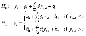
 is observed at discrete time points t. TAR(p), a TAR model of order p and two regimes can be written as
 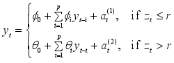 (1)
(1)  is the threshold variable, and
  are independent Gaussian white noise processes with mean zero and variance
  , with j = 1,2.
  and
and  are real-valued parameters and r is the threshold.
  value is replaced with previous values of the time series
  as below, the TAR model is then referred to as SETAR model.
 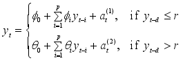 (2)
(2)  , that is,
  , where d represents the delay parameter.
  be a positive finite integer and
 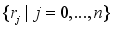 a real number sequence with
 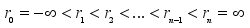 where
where  and
and  are regarded as real numbers. Then a time series
  is a m-regime SETAR (p) model if it satisfies
 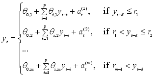 (3)
(3)  is the threshold variable and
  is the delay parameter.
  are collected of a time series
  . Suppose that each data point,
  , is associated with a probability distribution which can be expressed as a function of a parameter or many parameters
  so that the relationship between
  and
and  is described by a pdf
  . When
  is considered as a function of
  instead of
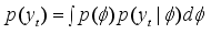
  , it is referred to as the likelihood function. By applying Bayes' theorem, the posterior pdf
  can be derived, that is, the posterior pdf of
  given
given  , by multiplying the likelihood with the prior density,
  . That is,
 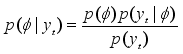 (4)
(4) 
 defines what is known as predictive density function. The prior distribution provides a means to include researcher's initial beliefs or assumptions regarding
  , and Bayes' theorem enables the revision and updating of these assumptions once the data is observed.
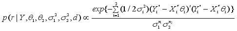
  and
and  are taken as independent and normally distributed as
  , while
  and
and  are taken as independent with inverse gamma distribution inverse gamma
 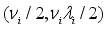 . The hyper-parameters d and r are assumed to be known. r is presumed to have a uniform distribution on
  while d is presumed to take a discrete uniform distribution on 1,2,..., D.
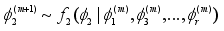
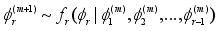
  's,
's,  s, r, and d. Determining the posterior distribution is frequently achallenging task due to the need for complex numerical integration in high-dimensional spaces. Therefore, Gibbs Sampler and the Metropolis-Hastings algorithm will be used in this study to find the conditional posterior distributions of the unknown parameters.
  can be broken down into components
  and the conditional densities
  can be simulated for
  . Then, to sample from the joint density of
  using Gibbs sampler, the following algorithm is followed:
  , generate
 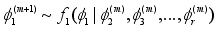 ,
,  ,
,  .
.  (5)
(5)  and
and  being functions of r.
  is made. Hence, a transition kernel
  with
with  can be utilized to map
  into
into  . The Metropolis algorithm will then work in the following manner;
  drawn from the prior
  and set the indicator
  to 0.
to 0.  , generate a new point
  .
.  , update
  to
to  and remain at
  with a probability of
  .
.  (6)
(6)  (hasunitroots)
  (nounitroots)
  (serieshasaunitrootwithdrift)
  (seriesisstationarywithbreak(s))
 Working Orders | Test statistic | P-value |
|---|---|---|
1 | 1.246 | 0.2652 |
2 | 1.871 | 0.1345 |
3 | 1.671 | 0.1276 |
4 | 1.59 | 0.1085 |
5 | 1.634 | 0.06407 |
6 | 2.272 | 0.001457 |
7 | 2.453 | 0.000116 |
8 | 2.273 | 0.0001182 |
9 | 2.18 | 8.27e-05 |
10 | 2.273 | 1.068e-05 |
P-values | ||||
|---|---|---|---|---|
Embedding Dimension | ε (standard deviation) | |||
0.5 | 1.0 | 1.5 | 2.0 | |
2 | 2.2 e-16 | 2.2 e-16 | 2.2 e-16 | 2.2 e-16 |
3 | 2.2 e-16 | 2.2 e-16 | 2.2 e-16 | 2.2 e-16 |
 .
.  are estimated using the Bayesian approach. The Gibbs sampler was executed for 1,000 iterations, and the initial 500 iterations were disregarded as the burn-in sample. The estimates of the parameters alongside their standard errors are as shown in the table below;
 Parameter | Mean | Median | Standard Deviation |
|---|---|---|---|
| -0.0332 | -0.0327 | 0.0109 |
| -0.2871 | -0.2894 | 0.1590 |
| 0.0739 | 0.0677 | 0.1353 |
| -0.0866 | -0.0818 | 0.1369 |
| 0.3277 | 0.3282 | 0.1194 |
| 0.0023 | 0.0020 | 0.0042 |
| 0.1288 | 0.1301 | 0.0963 |
| 0.0532 | 0.0566 | 0.0584 |
| 0.1191 | 0.1162 | 0.0593 |
| 0.0616 | 0.0607 | 0.0668 |
| 0.0033 | 0.0032 | 0.0005 |
| 0.0024 | 0.0024 | 0.0002 |
r | -0.0218 | -0.0215 | 0.0037 |
d | 1 | 1 | 0.0000 |
 and
and  . The estimated value of d is 1.
 Predictions | |||
|---|---|---|---|
Month/Year | Mean | Lower | Upper |
Sep 2024 | 1683.5889 | 1661.17926 | 1703.74326 |
Oct 2024 | 1689.9987 | 1667.50375 | 1711.25625 |
Nov 2024 | 1665.6705 | 1613.37418 | 1688.30953 |
Dec 2024 | 1671.6777 | 1645.47278 | 1692.53558 |
Jan 2025 | 1677.5389 | 1654.05153 | 1697.62081 |
Feb 2025 | 1684.2624 | 1661.51153 | 1707.66638 |
Mar 2025 | 1693.7208 | 1664.00567 | 1738.85656 |
Apr 2025 | 1698.9795 | 1676.19736 | 1719.14616 |
May 2025 | 1704.7658 | 1680.7292 | 1723.79413 |
June 2025 | 1713.6537 | 1685.10479 | 1753.52448 |
Jul 2025 | 1718.9743 | 1697.45106 | 1739.20437 |
Aug 2025 | 1723.9665 | 1700.33918 | 1743.90657 |
Bayesian SETAR | Frequentist SETAR | ARIMA | |
|---|---|---|---|
RMSE | 0.05074525 | 0.04949407 | 0.05102666 |
Bayesian SETAR | Frequentist SETAR | ARIMA | |
|---|---|---|---|
RMSE | 0.03947424 | 0.05351723 | 0.04191522 |
SETAR | Self-Exciting Threshold Autoregressive |
NSE | Nairobi Securities Exchange |
NSE20 | NSE 20 Share Index |
Probability Density Function | |
AR | Autoregressive |
MA | Moving Average |
ARIMA | Autoregressive Integrated Moving Average |
i.i.d | Independently and Identically Distributed |
| [1] | Tong H., Lim K. S., Threshold Autoregression, Limit Cycles and Cyclical Data. Journal of the Royal Statistical Society: Series B (Methodological). 1980, 42(3), 245-268. |
| [2] | Aydin D., Güneri Ö. İ. Time Series Prediction Using Hybridization of AR, SETAR and ARM Models. International Journal of Applied. 2015, 5(6), 87-96. |
| [3] | Boero G., Lampis F. The Forecasting Performance of SETAR Models: An Empirical Application. Bulletin of Economic Research. 2017, 69(3), 216-228. |
| [4] | Firat E. H. SETAR (Self-Exciting Threshold Autoregressive) Non-Linear Currency Modelling in EUR/USD, EUR/TRY and USD/TRY Parities. Mathematics and Statistics. 2017, 5(1), 33-55. |
| [5] | Gibson D., Nur D. Threshold Autoregressive Models in Finance: A Comparative Approach. In Proceedings of the Fourth Annual ASEARC Conference, University of Western Sydney, Paramatta, Australia, 2011; 18-23. |
| [6] | Oyewale A. M., Adelekan O. G., Innocient O. O. Forecast Comparison of Seasonal Autoregressive Integrated Moving Average (SARIMA) and Self Exciting Threshold Autoregressive (SETAR) Models. American Journal of Theoretical and Applied Statistics. 2017, 6(6), 278-283. |
| [7] | Tobechukwu N. M., Emmanuel B. O., Ibienebaka B. T. Self-Exciting Threshold Autoregressive Modelling of COVID-19 Confirmed Daily Cases in Nigeria. International Journal of Data Science and Analysis. 2022, 8(6), 182-186. |
| [8] | Agiwal V., Kumar, J. Bayesian Estimation for Threshold Autoregressive Model with Multiple Structural Breaks. Metron. 2020, 78(3), 361-382. |
| [9] | Ojo O. O. Bayesian Modelling of Inflation in Nigeria with Threshold Autoregressive Model. Rattanakosin Journal of Science and Technology. 2021, 3(1), 10-18. |
| [10] | Pan J., Xia Q., Liu J. Bayesian Analysis of Multiple Thresholds Autoregressive Model. Computational Statistics. 2017, 32, 219-237. |
| [11] | Onyeka-Ubaka J. N., Ebiringa O. A. Self-exciting Threshold Autoregressive Model with Application to Crude Oil Production in Nigeria. Asian Journal of Probability and Statistics. 2023, 22(1), 1-18. |
| [12] | Andric V., Bodroza D., Djukic M. A Commentary on US Sovereign Debt Persistence and Nonlinear Fiscal Adjustment. Mathematics. 2024, 12(20), 3250. |
| [13] | Bolstad W. M., Curran J. M. Introduction to Bayesian statistics. John Wiley & Sons. 2016, 237-253. |
| [14] | Bisaglia L., Canale A. Bayesian Nonparametric Forecasting for INAR Models. Computational Statistics & Data Analysis. 2016, 100, 70-78. |
| [15] | Drovandi C. C., Pettitt A. N., McCutchan R. A. Exact and Approximate Bayesian Inference for Low Integer-Valued Time Series Models with Intractable Likelihoods. 2016, 11(2) 325 - 352. |
| [16] | Li Y., Yu J., Zeng T. Deviance Information Criterion for Latent Variable Models and Misspecified Models. Journal of econometrics. 2020, 216(2), 450-493. |
| [17] | Yang K., Li H., Wang D. Estimation of Parameters in the Self-Exciting Threshold Autoregressive Processes for Nonlinear Time Series of Counts. Applied Mathematical Modelling. 2018, 57, 226-247. |
APA Style
Muindi, J., Muhua, G., Wanyonyi, R. (2024). Self-Exciting Threshold Autoregressive (SETAR) Modelling of the NSE 20 Share Index Using the Bayesian Approach. American Journal of Theoretical and Applied Statistics, 13(6), 203-212. https://doi.org/10.11648/j.ajtas.20241306.13
ACS Style
Muindi, J.; Muhua, G.; Wanyonyi, R. Self-Exciting Threshold Autoregressive (SETAR) Modelling of the NSE 20 Share Index Using the Bayesian Approach. Am. J. Theor. Appl. Stat. 2024, 13(6), 203-212. doi: 10.11648/j.ajtas.20241306.13
AMA Style
Muindi J, Muhua G, Wanyonyi R. Self-Exciting Threshold Autoregressive (SETAR) Modelling of the NSE 20 Share Index Using the Bayesian Approach. Am J Theor Appl Stat. 2024;13(6):203-212. doi: 10.11648/j.ajtas.20241306.13
@article{10.11648/j.ajtas.20241306.13,
  author = {Jacinta Muindi and George Muhua and Ronald Wanyonyi},
  title = {Self-Exciting Threshold Autoregressive (SETAR) Modelling of the NSE 20 Share Index Using the Bayesian Approach
},
  journal = {American Journal of Theoretical and Applied Statistics},
  volume = {13},
  number = {6},
  pages = {203-212},
  doi = {10.11648/j.ajtas.20241306.13},
  url = {https://doi.org/10.11648/j.ajtas.20241306.13},
  eprint = {https://article.sciencepublishinggroup.com/pdf/10.11648.j.ajtas.20241306.13},
  abstract = {The analysis and interpretation of time series data is of great importance across different fields, including economics, finance, and engineering, among other fields. This kind of data, characterized by sequential observations over time, sometimes exhibits complex patterns and trends that some commonly used models, such as linear autoregressive (AR) and simple moving average (MA) models, cannot capture. This limitation calls for the development of more sophisticated and flexible models that can effectively capture the complexity of time series data. In this study, a more sophisticated model, the Self-Exciting Threshold Autoregressive (SETAR) model, is used to model the Nairobi Securities Exchange (NSE) 20 Share Index, incorporating a Bayesian parameter estimation approach. The objectives of this study are to analyze the properties of the NSE 20 Share Index data, to determine the estimates of SETAR model parameters using the Bayesian approach, to forecast the NSE 20 Share Index for the next 12 months using the fitted model, and to compare the forecasting performance of the Bayesian SETAR with the frequentist SETAR and ARIMA model. Markov Chain Monte Carlo (MCMC) techniques, that is, Gibbs sampling and the Metropolis-Hastings Algorithm, are used to estimate the model parameters. SETAR (2; 4, 4) model is fitted and used to forecast the NSE 20 Share Index. The study's findings generally reveal an upward trajectory in the NSE 20 Share Index starting September 2024. Even though a slight decline is predicted in November, an upward trend is predicted in the following months. On comparing the performance of the models, the Bayesian SETAR model performed better than the linear ARIMA model for both short and longer forecasting horizons. It also performed better than its counterpart model, which uses the frequentist approach for a longer forecasting horizon. These results show the applicability of SETAR modeling in capturing non-linear dynamics. The Bayesian approach incorporated for parameter estimation advanced the model even further by providing a flexible and robust way of parameter estimation and accommodating uncertainty.
},
 year = {2024}
}
TY  - JOUR
T1  - Self-Exciting Threshold Autoregressive (SETAR) Modelling of the NSE 20 Share Index Using the Bayesian Approach

AU  - Jacinta Muindi
AU  - George Muhua
AU  - Ronald Wanyonyi
Y1  - 2024/11/26
PY  - 2024
N1  - https://doi.org/10.11648/j.ajtas.20241306.13
DO  - 10.11648/j.ajtas.20241306.13
T2  - American Journal of Theoretical and Applied Statistics
JF  - American Journal of Theoretical and Applied Statistics
JO  - American Journal of Theoretical and Applied Statistics
SP  - 203
EP  - 212
PB  - Science Publishing Group
SN  - 2326-9006
UR  - https://doi.org/10.11648/j.ajtas.20241306.13
AB  - The analysis and interpretation of time series data is of great importance across different fields, including economics, finance, and engineering, among other fields. This kind of data, characterized by sequential observations over time, sometimes exhibits complex patterns and trends that some commonly used models, such as linear autoregressive (AR) and simple moving average (MA) models, cannot capture. This limitation calls for the development of more sophisticated and flexible models that can effectively capture the complexity of time series data. In this study, a more sophisticated model, the Self-Exciting Threshold Autoregressive (SETAR) model, is used to model the Nairobi Securities Exchange (NSE) 20 Share Index, incorporating a Bayesian parameter estimation approach. The objectives of this study are to analyze the properties of the NSE 20 Share Index data, to determine the estimates of SETAR model parameters using the Bayesian approach, to forecast the NSE 20 Share Index for the next 12 months using the fitted model, and to compare the forecasting performance of the Bayesian SETAR with the frequentist SETAR and ARIMA model. Markov Chain Monte Carlo (MCMC) techniques, that is, Gibbs sampling and the Metropolis-Hastings Algorithm, are used to estimate the model parameters. SETAR (2; 4, 4) model is fitted and used to forecast the NSE 20 Share Index. The study's findings generally reveal an upward trajectory in the NSE 20 Share Index starting September 2024. Even though a slight decline is predicted in November, an upward trend is predicted in the following months. On comparing the performance of the models, the Bayesian SETAR model performed better than the linear ARIMA model for both short and longer forecasting horizons. It also performed better than its counterpart model, which uses the frequentist approach for a longer forecasting horizon. These results show the applicability of SETAR modeling in capturing non-linear dynamics. The Bayesian approach incorporated for parameter estimation advanced the model even further by providing a flexible and robust way of parameter estimation and accommodating uncertainty.

VL  - 13
IS  - 6
ER  -
Department of Mathematics, University of Nairobi, Nairobi, Kenya
Research Fields: Time Series Analysis and Forecasting, Bayesian Inference, Probability Modeling, Stochastic Processes, Survival Analysis and Epidemiology, Machine Learning
Department of Mathematics, University of Nairobi, Nairobi, Kenya
Research Fields: Time Series, Stochastic Processes, Sample Surveys, Statistical Modeling, Group Testing, Distribution Theory
Department of Mathematics, Egerton University, Nakuru, Kenya
Research Fields: Group Screening Designs & their Applications, Probability Modeling in Biological Processes, Multivariate and Inferential Statistics & Applications, Downscaling of Climate Outlook Forecasts, Times Series Analysis & Applications, Linear & Survival Models
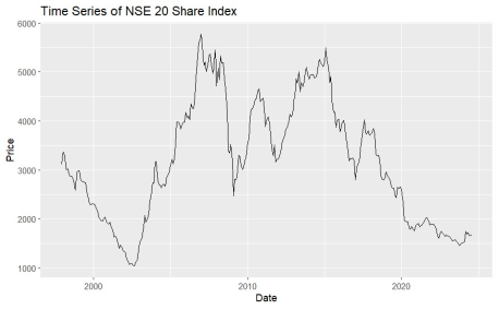
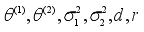
Figure 1. Time Series of NSE 20 share index monthly: Dec 1997 - Aug 2024.
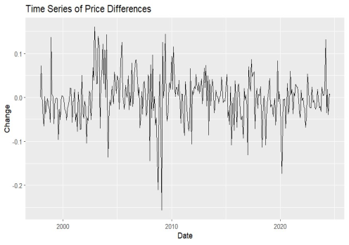
Figure 2. Time Series of Change in NSE 20 Share Index.
Figure 3. ACF Plot.
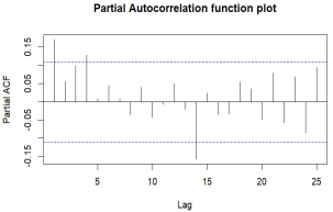
Figure 4. PACF Plot.
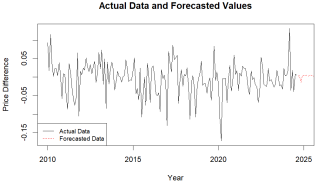
Figure 5. Predicted Future Changes of the NSE20 Index Are Indicated by the Red line.
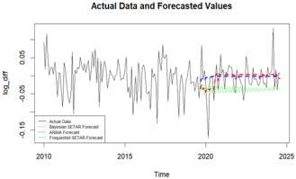
Figure 6. Original Data and Forecasted Values using Bayesian SETAR and using ARIMA.
Information


