Measuring Total Factor Productivity in General Technical Progress Framework

Lei Qinli

doi:doi:10.11648/j.ajtas.20241306.11

Research Article |

| Peer-Reviewed

Measuring Total Factor Productivity in General Technical Progress Framework

Lei Qinli^*

Published in American Journal of Theoretical and Applied Statistics (Volume 13, Issue 6)

Received: 7 October 2024 Accepted: 25 October 2024 Published: 12 November 2024

Views: Downloads:

Download PDF

Share This Article

Twitter
Linked In
Facebook

Abstract

The classical Solow's total factor productivity accounting assumes that technical progress is Hicks neutral, which is a special situation in the reality of world economy. This paper expands the setting of technical progress into general technical progress framework, which can cover Hicks neutral technical progress, Harrod neutral technical progress, Solow-neutral technical progress, and various factor-biased technical changes. According to the principle of statistical index number, this paper decomposes the output index into a total factor input index and a total factor productivity index, and adopts normalized CES production function with factor-augmenting technical progress to derive the calculation formulas of the total factor input index and the total factor productivity index, and constructs a new economic growth accounting system, and finds the counteraction and compensation mechanism for diminishing marginal returns. If the factor substitution elasticity is 1 or there is no technical progress bias and factor allocation bias, then the new accounting equation degenerates into the classic Solow growth accounting equation. The new accounting system can measure the influence of total factor input and total factor productivity to economic growth, but also can measure the influences of factor input intensity and factor allocation bias in the growth rate of total factor input, and the influences of technical progress intensity and technical progress bias in the growth rate of total factor productivity. Therefore it is more precise and accurate than classical method.

Published in	American Journal of Theoretical and Applied Statistics (Volume 13, Issue 6)
DOI	10.11648/j.ajtas.20241306.11
Page(s)	181-192
Creative Commons	This is an Open Access article, distributed under the terms of the Creative Commons Attribution 4.0 International License (http://creativecommons.org/licenses/by/4.0/), which permits unrestricted use, distribution and reproduction in any medium or format, provided the original work is properly cited.
Copyright	Copyright © The Author(s), 2024. Published by Science Publishing Group

Keywords

General Technical Progress, Economic Growth, Total Factor Input Index, Total Factor Productivity Index

1. Introduction

Total Factor Productivity (TFP) is the comprehensive productivity of all input factors in production process, reflecting the overall production efficiency of all input factors. TFP growth is a crucial source of economic growth and competitiveness. Statistical measurement of TFP growth is an important tool for assessing and monitoring economic performance, and constitutes core indicator for the analysis of economic growth.

The Solow

[20]

residual approach based on the neoclassical economic growth accounting equation is currently standard method for measuring TFP in statistical offices in the world. To this end, OECD

[18]

has published a measuring manual to guide the measurements of TFP in the OECD countries. However, the technological foundation of Solow growth accounting system is Hicks neutrality, which does not fully conform to economic reality, and the measure results are bound to have certain biases. Given the fact that technical progress is not neutral in the reality of economic development, Lei Qinli

[12]

derived a general formula for measuring biased technical progress based on a general form of production function with factor-augmenting technical progress. Dong Zhiqing and Chen Rui

[4]

, Lei Qinli and Xu Jiachun

[14]

, Yu Donghua and Chen Ruying

[21]

all followed the Solow classical continuous time total differentiation method to attempt to decompose various sources of economic growth, using aggregate Constant Elasticity of Substitution (CES) production function with factor-augmenting technical progress. Although these studies are based on the same type of production function, the calculation methods for total factor productivity are different. So where exactly does the problem lie? How can we solve the existing problems? Obviously, further exploration is needed.

Through in-depth consideration of the above issues, this article finds that the root of the problem lies in the difficulty of traditional continuous time differentiation methods in effectively decomposing the interaction between technical progress bias and factor allocation bias. Therefore, this article is based on general assumption framework of technical progress, which is different from the previous approach of using Solow continuous time differentiation method. Instead, this article constructs an economic growth index system according to the principle of discrete-time statistical index, gives the definitions of total factor input index and total factor productivity index, and then uses the normalized form of CES production function with general technical progress framework to derive the calculation formulas and decomposition methods of the total factor input growth index and total factor productivity growth index. Meanwhile, as a byproduct, this article also finds the compensation mechanism for the diminishing marginal returns of factors caused by the bias of technical progress towards capital deepening. Based on the new growth accounting model, this article also decomposes and calculates the annual economic growth of China since 1978-2019, and compares with traditional classical accounting methods.

2. A General Framework for Technical Progress

The setting of the production function is the starting point for economic growth accounting. The production function characterizes the combination of various production factors and production technologies in the production process, and describes the relationship between factor input and output. In economic theory, there are various settings regarding the combination of technology and production factors. Due to the different definitions of neutrality, in addition to Hicks neutral technical change, there are also Harrod neutral technical change and Solow neutral technical change. However, these neutral technical changes only capture a special situation in the real world. Hicks neutral technical change is independent of production factors, Harold neutral technical change is the type of purely labor augmenting progress, which has been used to analyze the mature economy; and Solow neutral technical change is the type of purely capital augmenting progress, which has been used to analyze the underdeveloped economy (Fei and Ranis

[5]

). In fact, in the process of real economic growth, technical changes are more likely to be biased towards particular factors, such as labor-biased technical change and capital-biased technical change. There are two major forces affecting equilibrium bias, the price effect encourages innovation directed at scarce bias, and the market size effect leads to technical change favoring abundant factors (Acemoglu

[1, 2]

). Therefore, in order to cover various types of technical progress in reality, it is necessary to construct a universal framework for technical progress. The so-called universal technical progress framework refers to a general technical progress framework that can include various types of neutral technical progress, as well as various particular factor-biased technical progresses. For this purpose, consider the general form of production function with factor augmenting technical progress:

Y = F (A^{K} K, A^{L} L)

(1)

Where,

Y

is total real output,

K

is capital input,

L

is labor input,

A^{K}

and

A^{L}

are technologies embodied in capital and labor, respectively. If

A^{K}

A^{L}

, then technology can be separated independently from production factors, and production function will be reduced as

Y = AF (K, L)

, with Hicks neutral technology; If

A^{L} \neq A^{K} = 1

, production function will be reduced as

Y = F (K, AL)

, with Harrods neutral technology; If

A^{K} \neq A^{L} = 1

, production function will be reduced as

Y = F (AK, L)

, with Solow neutral technology. Usually, there is

A^{K} \neq A^{L}

, then the general form of production function (1) can characterize various particular factor-biased technologies.

In order to perform practical accounting operations, a specific form of production function is required. Acemoglu's theoretical research showed that the Constant Elasticity of Substitution (CES) production function can well characterize biased technical changes, and de La Grandville

[3]

, Klump and de La Grandville

[7]

, and Klump and Preissler

[9]

presented that the aggregate CES production function can be much improved by normalization. A family of normalized CES production function has a common baseline point as comparison benchmark which can be any point on a CES function (Papageorgiou and Saam

[19]

), and its parameters then have a direct and clear economic meaning. Additionally, all variables in the production function can be transformed into index number forms, avoiding the influence of variable dimensions. The normalized CES production function with factor augmenting technical progress takes the form:

Y_{t} = Y_{0} {[α_{0} {(\frac{A_{t}^{K} K_{t}}{A_{0}^{K} K_{0}})}^{\frac{σ - 1}{σ}} + (1 - α_{0}) {(\frac{A_{t}^{L} L_{t}}{A_{0}^{L} L_{0}})}^{\frac{σ - 1}{σ}}]}^{\frac{σ}{σ - 1}}

(2)

Where

t

is time point,

t = 0

is the benchmark point.

Y_{0}

is output at the benchmark point,

α_{0} = r_{0} K_{0} / (r_{0} K_{0} + w_{0} L_{0})

is the income share of capital at the benchmark point,

r_{0}

and

w_{0}

are the rates of return of capital and wage of labor at the benchmark point respectively,

σ \in (0, \infty)

representing the substitution elasticity between capital and labor, and when

σ = 1

, the production function (2) degenerates into the Cobb-Douglas production function; when

σ = 0

, it degenerates into the Leontief production function; when

σ \to \infty

, then degenerates into the linear production function; therefore the CES production function nests various form of production functions.

Unlike the classical Cobb-Douglas production function where the income shares of capital and labor factors are constant, under the framework of CES production function with factor augmenting technical progress, both capital and labor income share are changing. For further analysis, take derivatives of capital and labor on both side of normalized CES production function (2), and obtain capital and labor marginal output as follows respectively:

\frac{\partial Y_{t}}{\partial K_{t}} = α_{0} \frac{Y_{0}}{K_{0}} {(\frac{A_{t}^{K}}{A_{0}^{K}})}^{\frac{σ - 1}{σ}} {(\frac{Y_{t} / Y_{0}}{K_{t} / K_{0}})}^{\frac{1}{σ}} = r_{0} {(\frac{A_{t}^{K}}{A_{0}^{K}})}^{\frac{σ - 1}{σ}} {(\frac{Y_{t} / Y_{0}}{K_{t} / K_{0}})}^{\frac{1}{σ}}

(3)

\frac{\partial Y_{t}}{\partial L_{t}} = (1 - α_{0}) \frac{Y_{0}}{L_{0}} {(\frac{A_{t}^{L}}{A_{0}^{L}})}^{\frac{σ - 1}{σ}} {(\frac{Y_{t} / Y_{0}}{L_{t} / L_{0}})}^{\frac{1}{σ}} = w_{0} {(\frac{A_{t}^{L}}{A_{0}^{L}})}^{\frac{σ - 1}{σ}} {(\frac{Y_{t} / Y_{0}}{L_{t} / L_{0}})}^{\frac{1}{σ}}

(4)

In a market economy of free competition, the rate of return of production factors is equal to their marginal output. Let

α_{t} = r_{t} K_{t} / Y_{t}

denote the income share of capital at

t

period, and let

β_{t} = (1 - α_{t}) = w_{t} L_{t} / Y_{t}

denote the income share of labor at

t

period. Then, from equations (3) and (4), the income share ratio of capital and labor can be obtained as:

π_{t} = \frac{α_{t}}{β_{t}} = \frac{α_{0}}{β_{0}} {(\frac{A_{t}^{K} K_{t} / A_{0}^{K} K_{0}}{A_{t}^{L} L_{t} / A_{0}^{L} L_{0}})}^{\frac{σ - 1}{σ}}

(5)

Acemoglu

[1]

defined the direction of technical progress in the sense that factor marginal rate of substitution changed by technical change. However, more appropriately, the direction of technical progress should be defined in the sense that factor income share ratio changed by technical change. From equation (5), it can be seen that the change in the ratio of capital to labor income share depends on two factors: one is the relative change between capital augmenting technology and labor augmenting technology; the second is the change in ratio of capital quantity to labor quantity, which ratio is also referred to as capital deepening. Therefore, the Technical Progress Bias Index can be defined as:

B_{t} = \frac{1}{π_{t}} \frac{\partial (α_{t} / β_{t})}{\partial (A_{t}^{K} / A_{t}^{L})} \frac{d (A_{t}^{K} / A_{t}^{L})}{dt} = (\frac{σ - 1}{σ}) (\frac{{\overset{́}{A}}_{t}^{K}}{A_{t}^{K}} - \frac{{\overset{́}{A}}_{t}^{L}}{A_{t}^{L}})

(6)

Adding a dot above the variable indicates the derivative of the variable with respect to time, i.e. the growth amount, for example

{\overset{́}{A}}_{t}^{K} = d A_{t}^{K} / dt

. If

B_{t} > 0

, technical changes result in an increase in the share of capital income relative to the share of labor income, then technical changes are biased towards capital; On the contrary, if

B_{t} < 0

, then technical changes are biased towards labor; If

B_{t} = 0

, technical changes do not alter the share of factor income, then technical changes are neutral.

Similarly, in order to measure the impact of capital deepening on changes in the ratio of capital to labor income share, the Capital Deepening Impact Index which is also referred as the Factor Allocation Bias Index can be defined as:

D_{t} = \frac{1}{π_{t}} \frac{\partial (α_{t} / β_{t})}{\partial (K_{t} / L_{t})} \frac{d (K_{t} / L_{t})}{dt} = (\frac{σ - 1}{σ}) (\frac{{\overset{́}{K}}_{t}}{K_{t}} - \frac{{\overset{́}{L}}_{t}}{L_{t}})

(7)

D_{t} > 0

, the change in factor allocation leads to an increase in the share of capital relative to labor income, the change in factor allocation is biased towards capital; On the contrary, if

D_{t} < 0

, then the change in factor allocation is biased towards labor; If

D_{t} = 0

, the change in factor allocation is neutral and does not affect the share of factor income.

Equations (6) to (7) indicate that both the direction of the technical progress bias index and the factor allocation bias index are closely related to the elasticity of factor substitution. When

σ > 1

, if the rate of improvement of the technology level embodied on capital is faster than that of the technology level embodied on labor, then technical progress is biased towards capital, and capital deepening is also biased towards capital; On the contrary, when

σ < 1

, if the rate of improvement of the technology level embodied on capital is faster than that of the technology level embodied on labor, then technical progress is biased towards labor, and capital deepening is also biased towards labor.

By taking the logarithm on both sides of the factor income share ratio equation (5) and taking the derivative over time, then obtain as:

\frac{{\overset{́}{π}}_{t}}{π_{t}} = \frac{{\overset{́}{α}}_{t}}{α_{t}} - \frac{{\overset{́}{β}}_{t}}{β_{t}} = (\frac{σ - 1}{σ}) [(\frac{{\overset{́}{A}}_{t}^{K}}{A_{t}^{K}} - \frac{{\overset{́}{A}}_{t}^{L}}{A_{t}^{L}}) + (\frac{{\overset{́}{K}}_{t}}{K_{t}} - \frac{{\overset{́}{L}}_{t}}{L_{t}})] = B_{t} + D_{t}

(8)

Because of

α_{t} + β_{t} = 1

, one of the factor income shares will increase while the other will inevitably decrease, but due to different base values, the increase rate of one and decrease rate of the other are not the same. The difference between the change rate of capital share and the change rate of labor share in equation (8) actually measures the total change rate of the two factor shares, while the right side of the equation indicates that the total change rate of the factor shares is completely determined by the technical progress bias index and the factor allocation bias index.

The current standard method for calculating total factor productivity based on the classic Solow growth accounting equation first uses the average of factor income shares in the base period and reporting period as a weight to calculate the total factor input growth rate, and then take the “surplus” obtained by subtracting the growth rate of total factor inputs from the total real output growth rate as the growth rate of total factor productivity. It is not difficult to see that the total factor input growth rate is also mixed with the influence of technical progress bias on factor income share, while the total factor productivity growth rate lacks the influence of technical progress bias. Therefore, the classical standard accounting method cannot accurately decompose the total factor input growth and productivity growth in economic growth.

3. Constructing Economic Growth Accounting Equation

According to economic theory, the growth of output depends on two factors: an increase in capital and labor input, and an improvement in production technology level. Therefore, if let

Y_{t}

denote the output in the

t

period, and let

Y_{t - 1}

denote the output in the

t - 1

period, then based on the index number system, under the general form of production function with factor augmenting technical progress, the Total Real Output (TRO) index can be decomposed into:

\frac{Y_{t}}{Y_{t - 1}} = \frac{F (A_{t}^{K} K_{t}, A_{t}^{L} L_{t})}{F (A_{t - 1}^{K} K_{t - 1}, A_{t - 1}^{L} L_{t - 1})} = \frac{F (A_{t - 1}^{K} K_{t}, A_{t - 1}^{L} L_{t})}{F (A_{t - 1}^{K} K_{t - 1}, A_{t - 1}^{L} L_{t - 1})}

\times \frac{F (A_{t}^{K} K_{t}, A_{t}^{L} L_{t})}{F (A_{t - 1}^{K} K_{t}, A_{t - 1}^{L} L_{t})} = \frac{{TFI}_{t}}{{TFI}_{t - 1}} \times \frac{{TFP}_{t}}{{TFP}_{t - 1}}

(9)

The first index on the right side of the equation (9) is the Total Factor Input (TFI) index, which reflects the impact of changes in factor inputs on output; the second index is the Total Factor Productivity (TFP) index, which reflects the impact of technical progress on output.

For the convenience of calculation, referring to the methods of Klump et al.

[8]

and Leon-Ledesma et al.

[17]

, taking the logarithm of the CES production function with factor augmenting technical progress (2), and using Kmenta’s

[10]

second-order Taylor series expansion, then obtain as follow:

\ln (\frac{Y_{t}}{Y_{0}}) = α_{0} \ln (\frac{A_{t}^{K} K_{t}}{A_{0}^{K} K_{0}}) + β_{0} \ln (\frac{A_{t}^{L} L_{t}}{A_{0}^{L} L_{0}})

\frac{α_{0} β_{0}}{2} \frac{σ - 1}{σ} {[\ln (\frac{A_{t}^{K} K_{t}}{A_{0}^{K} K_{0}}) - \ln (\frac{A_{t}^{L} L_{t}}{A_{0}^{L} L_{0}})]}^{2}

(10)

Applying formula (10) to the decomposition equation of the total output index (9) and simplifying it, the logarithmic formulas for the total factor input index and total factor productivity index are obtained as follows:

\ln (\frac{{TFI}_{t}}{{TFI}_{t - 1}}) = \ln (\frac{F (A_{t - 1}^{K} K_{t}, A_{t - 1}^{L} L_{t})}{F (A_{t - 1}^{K} K_{t - 1}, A_{t - 1}^{L} L_{t - 1})})

= α_{0} \ln (\frac{K_{t}}{K_{t - 1}}) + β_{0} \ln (\frac{L_{t}}{L_{t - 1}}) + α_{0} β_{0} (\frac{σ - 1}{σ})

\{\ln (\frac{A_{t - 1}^{K} K_{t - 1} / A_{0}^{K} K_{0}}{A_{t - 1}^{L} L_{t - 1} / A_{0}^{L} L_{0}}) + \frac{1}{2} [\ln (\frac{K_{t}}{K_{t - 1}}) - \ln (\frac{L_{t}}{L_{t - 1}})]\}

[\ln (\frac{K_{t}}{K_{t - 1}}) - \ln (\frac{L_{t}}{L_{t - 1}})]

(11)

\ln (\frac{{TFP}_{t}}{{TFP}_{t - 1}}) = \ln (\frac{F (A_{t}^{K} K_{t}, A_{t}^{L} L_{t})}{F (A_{t - 1}^{K} K_{t}, A_{t - 1}^{L} L_{t})})

= α_{0} \ln (\frac{A_{t}^{K}}{A_{t - 1}^{K}}) + β_{0} \ln (\frac{A_{t}^{L}}{A_{t - 1}^{L}}) + α_{0} β_{0} (\frac{σ - 1}{σ})

\{\ln (\frac{A_{t}^{K} K_{t} / A_{0}^{K} K_{0}}{A_{1}^{L} L_{t} / A_{0}^{L} L_{0}}) + \frac{1}{2} [\ln (\frac{A_{t}^{K}}{A_{t - 1}^{K}}) - \ln (\frac{A_{t}^{L}}{A_{t - 1}^{L}})]\}

[\ln (\frac{A_{t}^{K}}{A_{t - 1}^{K}}) - \ln (\frac{A_{t}^{L}}{A_{t - 1}^{L}})]

(12)

Using the factor income share ratio

π_{t}

in equation (5) and the technological progress bias index

B_{t}

in equation (6) and the factor allocation bias index

D_{t}

in equation (7), and using mathematical approximation equation

\ln (X_{t} / X_{t - 1}) = \ln (1 + {∆ X}_{t} / X_{t - 1}) \approx {∆ X}_{t} / X_{t - 1}

, in which

∆ X_{t} = X_{t} - X_{t - 1}

and

|∆ X_{t}| / X_{t - 1}

is small, then from equations (11) and (12). there can obtain the growth rate index of total factor input and the growth rate index of total factor productivity, which are respectively:

\frac{∆ {TFI}_{t}}{{TFI}_{t - 1}} = (α_{0} \frac{∆ K_{t}}{K_{t - 1}} + β_{0} \frac{∆ L_{t}}{L_{t - 1}}) +

α_{0} β_{0} [\ln (\frac{π_{t - 1}}{π_{0}}) + \frac{1}{2} D_{t}] (\frac{∆ K_{t}}{K_{t - 1}} - \frac{∆ L_{t}}{L_{t - 1}}) = {FII}_{t} + {FBI}_{t}

(13)

\frac{∆ {TFP}_{t}}{{TFP}_{t - 1}} = (α_{0} \frac{∆ A_{t}^{K}}{A_{t - 1}^{K}} + β_{0} \frac{∆ A_{t}^{L}}{A_{t - 1}^{L}}) +

α_{0} β_{0} [\ln (\frac{π_{t}}{π_{0}}) - \frac{1}{2} B_{t}] (\frac{∆ A_{t}^{K}}{A_{t - 1}^{K}} - \frac{∆ A_{t}^{L}}{A_{t - 1}^{L}}) = {TPI}_{t} + {TBI}_{t}

(14)

Equations (13) and (14) provide the calculation formulas for the Total Factor Input Growth (TFIG) Index and the Total Factor Productivity Growth (TFPG) Index, respectively. Equation (13) indicates that the total factor input growth rate index consists of two parts: one is the weighted average of the growth rates of capital and labor inputs, which is the pure factor input growth rate; the other is the impact of factor allocation bias, namely the impact of capital deepening. The former can be called the Factor Input Intensity (FII) Index, while the latter can be called the Factor Bias Impact (FBI) Index or the Capital Deepening Impact Index. Equation (14) indicates that the total factor productivity growth rate index also consists of two parts: one is the weighted average of the technical progress rates embodied in capital and labor, which is the pure technical progress intensity growth rate; the other is the impact of technical progress bias. Similarly, the former can be called the Technical Progress Intensity (TPI) Index, while the latter can be called the Technical Bias Impact (TBI) Index.

And from equation (9), there is the identity equation as follow:

\frac{∆ Y_{t}}{Y_{t - 1}} = \frac{∆ {TFI}_{t}}{{EFI}_{t - 1}} + \frac{∆ {TF P}_{t}}{{TFP}_{t - 1}}

(15)

In this Equation, the left side is Total Real Output Growth (TROG) index, and the right side is Total Factor Input Growth (TFIG) index and Total Factor Productivity Growth (TFPG) index. Therefore the equation indicates that economic growth consists of two parts: the growth of total factor inputs and the growth of total factor productivity.

According to the production theory in neoclassical economics, the production function

Y = F (K, L, A)

not only needs to have the property of constant returns to scale, but also must satisfy two mathematical properties: firstly, for all points with

K > 0

and

L > 0

, there are

F_{K} > 0

F_{L} > 0

; and

F_{KK} < 0

F_{LL} < 0

. All first-order derivatives are greater than 0, which reflect that the marginal product of each production factor input is positive; and each second-order derivatives is less than 0, which means that the marginal return on each factor of production input decreases. Secondly, Inada conditions: there must be

\lim_{K \to 0} F_{K} = \lim_{L \to 0} F_{L} = \infty

, and

\lim_{K \to \infty} F_{K} = \lim_{L \to \infty} F_{L} = 0

. Therefore, if the production function is transformed into an intensive form, that is transformed into per capita form:

y = F (K / L, A) = f (k, A)

, where

y = Y / L

is per capita output and

k = K / L

per capita capital, then there must be properties:

f_{k} > 0

f_{kk} < 0

, and

\lim_{k \to 0} f_{k} = \infty

\lim_{k \to \infty} f_{k} = 0

. This indicates that due to the law of diminishing marginal output, as per capita capital increases, the effect of capital input on output growth will become weaker, that is, the role of capital deepening in economic growth will continue to decline with its degree of deepening.

The historical practices of economic development in various countries around the world have shown that economic development is inevitably accompanied by the continuous accumulation of capital. Capital accumulation consists of two parts: capital widening and capital deepening. Capital widening equips new workers with new capital, while capital deepening increases the per capita capital. The process of economic growth is also the process of continuous deepening of capital. In the early stage of a country's economic development, there are usually abundance of labor and severe shortage of capital, and both per capita income and savings rate are very low, and new investment is insufficient to absorb excess labor, resulting in capital investment mainly being used for capital widening. When the economic development enters the takeoff stage, with the gradual digestion of surplus labor and the continuous improvement of per capita income, the savings rate and investment rate will continue to increase, capital deepening accelerates; When society enters the high-income stage, economic growth will approach its steady-state balanced growth path, unless there is technological innovation driving it, the benefits of new investment will continue to decline, capital deepening will continue to slow down or even stagnate. Therefore, the negative effects of capital deepening on output growth may not be apparent in the early stages of economic development, but will become apparent in the later stages of high-speed economic development. However, for developed economies that are close to the steady-state balanced growth path, due to the basic stagnation of capital deepening, its impact effect becomes smaller.

Due to the law of diminishing marginal returns, in the absence of technical progress, capital deepening has a restraining effect on output growth. But if accompanied by technological innovation and upgrading, the new investment is used to increase new equipment and machineries of enterprises, the capital deepening will lead to an increase in the demand for skilled labor, resulting in an increase in the proportion of skilled labor. Because the complementary effect of capital to skilled labor (Lei Qinli and Li Yuelin

[15]

), technical progress biased towards skilled labor tends to have an enhancing effect on economic growth. Therefore, it can be considered that the positive effect of the bias of technical progress on output growth is a counteraction to the diminishing marginal returns of capital deepening. That is to say, the positive effect of the skilled-labor-biased technical progress on output growth provide a compensation mechanism for the negative inhibitory effect of capital deepening on output growth caused by the law of diminishing marginal returns of capital.

Obviously, the new accounting formula is presented within a more realistic general framework of technical progress, covering multiple types of technical progress, and therefore has broad applicability. From equations (13) to (14), it can be seen that if the factor substitution elasticity is 1, the CES production function degenerates into the Cobb-Douglas production function; Or if there are no biases in technical progress and factor allocation, that is, the technical progress rates embodied in capital and labor are equal, and the factor allocation ratio of capital and labor remains unchanged, then the new accounting formula degenerates into the classical Solow residual formula. Therefore, Solow residual method is only a special case of the new accounting method. If equations (13) and (14) are added together, they form the decomposition accounting equation (15) for the growth rate of total output growth, which is consistent with the economic growth accounting equation derived by Lei Qinli

[13]

using the total differential method under continuous time conditions. However, the difference is that the new accounting equation given in this paper under discrete time conditions is more refined, and the inhibitory effect of capital deepening on economic growth and the promoting effect of technical progress bias on economic growth can be calculated separately through the factor allocation bias index and the technical progress bias index, thus making the accounting analysis more refined and accurate.

4. Factor Substitution Elasticity and Technical Progress Indices

To calculate the changes of total factor input and total factor productivity using equations (13) to (14), it is necessary firstly to calculate the change rates of capital and labor inputs, as well as the change rates of technology levels embodied in capital and labor. If the depth parameter of the production function – the factor substitution elasticity - is known or estimated in advance, then let the return rate of capital at

t

period be equal to the capital marginal output in the equation (3), and let the wage rate of labor at

t

period be equal to the labor marginal output in the equation (4), the technical progress indices of technology levels embodied in capital and labor based on a fixed point can be derived as follow:

\frac{A_{t}^{K}}{A_{0}^{K}} = {(\frac{r_{t}}{r_{0}})}^{\frac{σ}{σ - 1}} {(\frac{Y_{t} / Y_{0}}{K_{t} / K_{0}})}^{\frac{1}{1 - σ}} = {(\frac{α_{t}}{α_{0}})}^{\frac{σ}{σ - 1}} (\frac{Y_{t} / Y_{0}}{K_{t} / K_{0}})

(16)

\frac{A_{t}^{L}}{A_{0}^{L}} = {(\frac{w_{t}}{w_{0}})}^{\frac{σ}{σ - 1}} {(\frac{Y_{t} / Y_{0}}{L_{t} / L_{0}})}^{\frac{1}{1 - σ}} = {(\frac{β_{t}}{β_{0}})}^{\frac{σ}{σ - 1}} (\frac{Y_{t} / Y_{0}}{L_{t} / L_{0}})

(17)

After calculating the technical progress indices of technology levels embodied in capital and labor based on a fixed point in each reporting period using equations (16) to (17), the fixed-base index of each period can be divided by the fixed-base index of the previous period to obtain the chain index for each period. Based on this method, the chain change rate of the technological level embodied in capital and labor for each period can be calculated.

In order to estimate the factor substitution elasticity

σ

, based on the fact that the factor return rate in the competitive market economy is equal to its marginal output, then assuming that both changes of the technology levels embodied in capital and labor exhibit exponential changes with stochastic shocks, That is assuming

A_{t}^{K} = A_{0}^{K} e^{δ_{K} + γ_{K} (t - t_{0}) + ϵ_{Kt}}

and

A_{t}^{L} = A_{0}^{L} e^{δ_{L} + γ_{L} (t - t_{0}) + ϵ_{Lt}}

, where

γ_{K}

and

γ_{L}

are the average growth rates of technology levels embodied in capital and labor respectively,

ε_{Kt}

and

ε_{Lt}

are the random shocks, while setting constant terms

δ_{K}

and

δ_{L}

is to consider that due to differences in dimensions, the values of technology level embodied in capital and labor at the benchmark period may be different. The transformation of marginal output equations (3) to (4) for capital and labor yields a system of equations:

\ln (\frac{Y_{t} / Y_{0}}{K_{t} / K_{0}}) = δ_{K} (1 - σ) + γ_{K} (1 - σ) (t - t_{0})

+ σln (\frac{r_{t}}{r_{0}}) + (1 - σ) ε_{Kt}

(18)

\ln (\frac{Y_{t} / Y_{0}}{L_{t} / L_{0}}) = δ_{L} (1 - σ) + γ_{L} (1 - σ) (t - t_{0})

+ σln (\frac{w_{t}}{w_{0}}) + (1 - σ) ε_{Lt}

(19)

The reason for setting the capital productivity and labor productivity indices as the dependent variables and the return index of capital and labor as the explanatory variables is that the return rates of capital and labor are determined by the supply and demand relationship of the capital and labor markets, respectively. Even enterprises with a certain degree of monopoly power cannot determine the interest rate of capital and wage rate of labor in the market. The decisions that enterprises can make are only based on the price levels of capital and labor formed in the market, and determine how much capital to use, how much labor to hire, and how many products to produce. Therefore, capital and labor productivity are dependent variables, while capital and labor price levels are independent variables. Obviously, the coefficient of the logarithm of capital return index in equation (18) is the same as the coefficient of the logarithm of labor wage index in equation (19), which is

σ

, the elasticity of substitution between capital and labor. Therefore, a constrained system estimation method is needed to estimate this system of equations. Due to the fact that factor substitution elasticity is a deep parameter of the economic system, its value mainly is determined by social institutions, economical structure and cultural traditions (Lei Qinli

[12]

). The stability of institutions and cultural traditions and the slow change in industrial structure ensures that it is stable for a considerable period of time. Therefore, a time series sample of a country or region can be used for estimation.

If a time series sample with n periods of data has been obtained, the sample data of the dependent and explanatory variables in equations (18) and (19) can be stacked to form a 2n dimensional dependent variable data vector and a

2 n \times 5

-dimensional explanatory variable data matrix, respectively, and the random shock variables in the two equations can also be stacked to form a 2n dimensional stochastic disturbance vector. That is, Let matrices Z, X, and u be as follows:

Z = (\begin{matrix} \ln (\frac{Y_{t} / Y_{0}}{K_{t} / K_{0}}) \\ \ln (\frac{Y_{t} / Y_{0}}{L_{t} / L_{0}}) \end{matrix})

X = (\begin{matrix} \begin{matrix} 1_{n} & 0_{n} & t - t_{0} \\ 0_{n} & 1_{n} & 0_{n} \end{matrix} & \begin{matrix} 0_{n} & \ln (r_{t} / r_{0}) \\ t - t_{0} & \ln (w_{t} / w_{0}) \end{matrix} \end{matrix})

u = (\begin{matrix} (1 - σ) ϵ_{Kt} \\ (1 - σ) ϵ_{Lt} \end{matrix})

Where

1_{n}

is the vector which all elements equal to 1, and

0_{n}

is the vector which all elements equal to 0. Meanwhile, arrange the regression coefficients in equations (18) and (19) into a 5-dimensional coefficient vector

\emptyset

as:

\emptyset = (\begin{matrix} δ_{k} (1 - σ) & δ_{L} (1 - σ) & \begin{matrix} γ_{K} (1 - σ) & γ_{L} (1 - σ) & σ \end{matrix} \end{matrix})'

Using these matrices and vectors, the linear system of equation (18) and (19) can be concisely represented as:

Z = X∅ + u

(20)

Obviously, the equation (20) can be estimated using the systems ordinary least squares (SOLS) method. However, in reality, when external random events impact technological level embodied in capital, they may also have an impact on technological level embodied in labor. Therefore, the random errors

ε_{Kt}

and

ε_{Lt}

probably have contemporaneous correlation. Given correlation of the components of the error vector in equation (20) for a given period, more efficient estimation is possible by systems general least squares (SGLS) or systems feasible general least squares (SFGLS) method. For the tth period, denoting the

2 \times 2

covariance matrix of the disturbance in equation (20) is

Ω_{t} = E (u_{t} u_{t}^{'} | X_{t})

, and assuming

Ω_{t}

does not vary over t:

Ω_{t} = Ω

, then the SGLS estimator of the coefficient vector

ϕ

\hat{ϕ} = {[X' (Ω^{- 1} ⨂ I_{n}) X]}^{- 1} X' (Ω^{- 1} ⨂ I_{n}) Z

(21)

Where

I_{n}

denotes a

n \times n

identity matrix, and

⨂

denotes Kronecker product.

In practical applications, the contemporaneous covariance matrix

Ω

is usually unknown, so it is necessary to first use systems ordinary least squares method to estimate the covariance matrix, and then use systems generalized least squares method to estimate the regression coefficient vector, that is, use systems feasible generalized least squares method for estimation

5. Accounting Economic Growth in China

Based on the latest macroeconomic statistics released by the 2021 Statistical Yearbook of the National Bureau of Statistics, this article selects the period from 1978 to 2019 as the sample period to measure and analyze the changes of total factor productivity at the level of national economic aggregate output in China.

The output and factor input indicators are: the annual gross domestic product (GDP) is the final output, the annual average number of employed people is the labor input, and the annual average fixed capital stock is the capital input. In order to eliminate the impact of price fluctuations, the annual Gross Domestic Product (GDP) is converted from nominal GDP at current prices to real GDP at constant price, which is 2000 year price, through an implicit GDP deflator index series. The stock of fixed capital is estimated using the Perpetual Inventory Method (PIM). Firstly, data on nominal gross fixed capital formation, fixed capital investment price index, and depreciation rate of fixed assets over the years since 1953 are collected. The nominal fixed capital formation for each year is converted to real fixed capital formation series at 2000 year fixed price using the fixed capital investment price index series. Then, based on the real fixed capital formation series from 1953 to 1978 and its annual average growth rate and average depreciation rate, the real fixed capital stock for the initial year 1978 is estimated using formula

K_{0} = I_{0} (1 + g) / (δ + g)

where

I_{0}

is real fixed asset formation at initial year,

δ

is the average of depreciation rate, and

g

is the average growth rate of real fixed asset investment from 1953 to 1978. Finally, the real fixed capital stock for each year is recursively calculated using PIM formula,

K_{t} = I_{t} + (1 - δ) K_{t - 1}

. Considering that with the widespread use of electronic devices, the depreciation period of fixed assets gradually shortens and depreciation accelerates, the sample is divided into three periods of 1978-1991, 1992-2001, and 2002-2019, and based on economic census data, the fixed asset depreciation rates for the three periods are set at 5.5%, 6.5%, and 7.5%, respectively (Lei Qinli

[11]

). The average number of employed people per year is calculated by taking the simple arithmetic mean of the number of employed people at the end of the current year and the end of the previous year. Considering that the employment data after 1990 in the China Statistical Yearbook has been revised several times based on population census and sampling survey data, and the data before 1990 has not been revised, there is a huge gap between the data of 1989 and 1990. Therefore, an adjustment ratio is calculated based on the employment numbers in 1990 and the adjusted employment numbers published in the original statistical yearbook, and the year-end employment numbers before 1990 are adjusted according to this adjustment ratio. Then, the capital productivity is obtained by dividing the annual real gross domestic product by the real fixed capital stock at 2000 price for each year; The labor productivity is obtained by dividing the annual real gross domestic product by the average number of employed people in each year.

The factor return rate and factor income share are calculated using the flow of funds accounts (non-financial transactions) table and the gross domestic product accounts from the perspective of income. The China Statistical Yearbook 2012 released the revised flow of funds accounts table for 2000-2009 years. Each yearbook after 2012 published the flow of funds accounts table for the previous year, but the latest 2021 yearbook published only the flow of funds accounts table for 2019. Due to the lack of the flow of funds accounts table before 2000, the GDP accounts from the perspective of income for each province in the "Historical Data of China's Gross Domestic Product Accounting 1952-1995" and "Historical Data of China's Gross Domestic Product Accounting 1952-2004" edited and published by the National Economic Accounting Department of the National Bureau of Statistics were used. From the perspective of income, the gross domestic product refers to the sum of all kinds of revenue, including compensation of employees, net taxes on production, depreciation of fixed assets, and operating surplus. Summing up the income data for each province separately yields the national income data for all categories. And distribute the net taxes on production proportionally to compensation of employees and operating surplus, then calculate the proportion of total compensation of employees to GDP each year to obtain the share of labor income for each year. Adding up the depreciation of fixed assets and operating surplus each year yields the total annual capital income, and calculating the proportion of total annual capital income to GDP yields the annual share of capital income. Then multiply the capital income share and labor income share of each year by the real GDP at 2000 price to obtain the total real capital return and labor return for each year. Finally, the labor return rate is obtained by dividing the total real labor income by the average annual number of employees, and the capital return rate is obtained by dividing the total real capital income by the real fixed capital stock,.

Looking back at the history since the reform and opening up, there was a clear turning point in the development of China's economy around 1992. From 1978 to 1992, China's economic system was dominated by a planned economy, supplemented by market regulation, and operated within the framework of a planned commodity economy based on public ownership. In the spring of 1992, Deng Xiaoping delivered a speech during his southern tour, and in October of the same year, the 14th National Congress of the Communist Party of China was held, which established the reform goal of building a socialist market economy system. This accelerated the pace of China's reform and opening up, and significantly accelerated economic development. For this purpose, a dummy variable is set up with 1992 as the boundary, with values of 0 for each year before 1992 and 1 for each year after 1992, to reflect the accelerated changes in economic development.

Considering that the global financial and economic crisis triggered by the US subprime mortgage crisis since 2007 has continued to spread and still has a significant impact, a dummy variable is also set, with a value of 0 for each year before 2007 and 1 for each year after 2007, to reflect changes in the world economic environment and situation.

Add the two dummy variables mentioned above to the linear systems of equations (18) and (19) respectively, and use the constrained system least squares method to estimate the parameters. The estimation results are shown in Table 1. It can be seen that the estimated coefficients of all explanatory variables are highly significant, and the estimated value of factor substitution elasticity is 0.48. In recent years, there have been many estimates and calculations of factor substitution elasticity in literatures. Leon-Ledesna et al.

[16]

reviewed the empirical studies on the substitution elasticity and technical bias in USA, and found the estimated values of substitution elasticity between capital and labor in USA are mostly 0.5 around. Hao Feng and Sheng Weiyan

[6]

reviewed the estimation results in China, and found that China's factor substitution elasticity is between 0.32 and 0.55. Therefore, it can be considered that the estimated value of 0.48 for China's capital and labor substitution elasticity given in Table 1 is reliable.

Table 1. Estimation of the Linear Systems of Equations.

Equations	$δ_{k} (1 - σ)$	$δ_{L} (1 - σ)$	$σ$	$D_{92}$	$D_{92} (t - t_{0})$	$D_{07}$	$D_{92} (t - t_{0})$	$R^{2}$
(18)	0.0312	0.0079	0.4815	0.2299	-0.0133	0.2844	-0.0109	0.9827
(18)	[0.0108]	[0.0015]	[0.0681]	[0.0432]	[0.0023]	[0.1082]	[0.0034]	0.9827
(19)	-0.0333	0.0325	0.4815	-0.0929	0.0103	0.3050	-0.0074	0.9995
(19)	[0.0105]	[0.0046]	[0.0681]	[0.0329]	[0.0021]	[0.0703]	[0.0022]	0.9995

Note: Standard Errors in parenthesis.

Based on the estimated values of factor substitution elasticity given in Table 1, the method proposed in this paper was used to calculate the changes in total factor productivity in China over the years. The calculation results are shown in Table 2. Firstly, columns 2-4 represent the annual GDP growth rate and the growth rate of capital and labor input, respectively, as the basic data for calculation and analysis. Secondly, columns 5-6 represent the annual change rates of technology levels embodied in capital and labor calculated using equations (16) to (17), while columns 7-8 represent the annual indices of technical progress bias and factor allocation bias calculated using equations (6) to (7). The following columns are the decomposition accounting of China's annual economic growth rate using the new accounting method proposed in this article. Columns 9-11 represent the total factor input intensity index, factor allocation bias impact index, and total factor input growth rate index, while columns 12-14 represent the technical progress intensity index, technical progress bias impact index, and total factor productivity growth rate index. Finally, column 15 represents the contribution rate of the total factor productivity growth rate calculated by the new method to economic growth.

Table 2. Accounting Economic Growth in China.

year	GDP	Factor		Technology		Bias Index		Economic Growth Accounting (%)
(1)	$\frac{∆ Y_{t}}{Y_{t - 1}}$	$\frac{∆ K_{t}}{K_{t - 1}}$	$\frac{∆ L_{t}}{L_{t - 1}}$	$\frac{∆ A_{t}^{K}}{A_{t - 1}^{K}}$	$\frac{∆ A_{t}^{L}}{A_{t - 1}^{L}}$	$B_{t}$	$D_{t}$	FII	FBI	$\frac{∆ {TFI}_{t}}{{TFI}_{t - 1}}$	TPI	TBI	$\frac{∆ {TFP}_{t}}{{TFP}_{t - 1}}$	$\frac{g_{TFP}}{g_{GDP}}$
1979	7.59	3.81	2.07	8.09	2.23	-6.35	-1.89	2.82	0.00	2.82	4.75	-0.05	4.70	61.86
1980	7.83	7.54	2.72	-0.76	5.76	7.06	-5.22	4.80	-0.11	4.69	2.95	0.14	3.09	39.42
1981	5.11	7.02	3.24	2.45	-1.12	-3.87	-4.09	4.86	-0.07	4.80	0.41	-0.09	0.33	6.43
1982	9.02	6.84	3.41	4.31	3.90	-0.44	-3.72	4.88	-0.11	4.77	4.08	-0.01	4.06	45.06
1983	10.77	7.25	3.05	3.14	7.59	4.82	-4.55	4.85	-0.18	4.68	5.68	0.19	5.87	54.46
1984	15.19	8.36	3.16	7.20	11.06	4.18	-5.62	5.40	-0.22	5.17	9.40	0.17	9.57	62.99
1985	13.43	9.93	3.63	1.65	10.53	9.61	-6.82	6.34	-0.30	6.04	6.71	0.41	7.11	52.97
1986	8.95	10.66	3.15	-1.59	5.66	7.86	-8.14	6.38	-0.33	6.05	2.54	0.31	2.85	31.88
1987	11.66	10.48	2.88	-1.42	10.36	12.76	-8.24	6.15	-0.33	5.82	5.29	0.47	5.76	49.44
1988	11.22	10.24	2.93	1.05	7.94	7.47	-7.92	6.08	-0.25	5.83	4.97	0.23	5.21	46.41
1989	4.21	7.87	2.38	-3.61	1.94	6.01	-5.95	4.74	-0.18	4.56	-0.45	0.17	-0.27	-6.51
1990	3.92	5.36	2.19	4.32	-1.98	-6.82	-3.43	3.55	-0.09	3.47	0.73	-0.23	0.50	12.75
1991	9.26	5.47	1.84	0.05	9.73	10.48	-3.93	3.40	-0.18	3.22	5.56	0.43	6.00	64.76
1992	14.22	6.54	1.08	1.01	17.78	18.18	-5.92	3.43	-0.21	3.21	10.57	0.53	11.09	77.99
1993	13.88	8.42	1.00	0.25	16.80	17.93	-8.04	4.19	-0.14	4.05	9.68	0.21	9.89	71.22
1994	13.04	10.01	0.98	5.83	9.44	3.92	-9.78	4.86	-0.02	4.84	7.89	0.03	7.91	60.69
1995	10.95	10.48	0.94	4.18	7.04	3.10	-10.34	5.04	-0.14	4.90	5.81	0.06	5.87	53.56
1996	9.92	10.55	1.10	-0.15	8.40	9.27	-10.24	5.17	-0.28	4.89	4.72	0.25	4.98	50.15
1997	9.24	10.23	1.28	-0.11	7.26	7.98	-9.70	5.13	-0.27	4.86	4.09	0.23	4.32	46.74
1998	7.85	10.25	1.22	-1.71	6.20	8.57	-9.79	5.10	-0.30	4.80	2.80	0.27	3.06	39.03
1999	7.66	10.11	1.12	-3.66	7.57	12.17	-9.74	4.99	-0.32	4.67	2.74	0.36	3.10	40.49
2000	8.49	9.75	1.02	1.98	5.12	3.40	-9.45	4.77	-0.25	4.52	3.77	0.11	3.88	45.67
2001	8.34	10.00	0.98	-2.52	8.04	11.44	-9.77	4.86	-0.37	4.49	3.49	0.42	3.91	46.90
2002	9.13	10.08	0.82	3.56	5.18	1.76	-10.02	4.81	-0.35	4.46	4.48	0.07	4.55	49.86
2003	10.04	10.81	0.64	-1.96	10.24	13.22	-11.02	5.02	-0.56	4.46	4.99	0.65	5.64	56.17
2004	10.11	11.94	0.67	-8.00	14.51	24.39	-12.21	5.52	-0.59	4.93	4.82	0.93	5.76	56.91
2005	11.39	12.36	0.62	-1.77	11.46	14.34	-12.72	5.67	-0.32	5.35	5.77	0.34	6.10	53.56
2006	12.72	12.56	0.48	-3.29	15.17	20.00	-13.09	5.68	-0.29	5.39	7.22	0.34	7.57	59.49
2007	14.23	12.94	0.45	-1.04	15.69	18.13	-13.54	5.83	-0.13	5.69	8.49	0.13	8.62	60.54
2008	9.65	13.08	0.39	-4.57	10.65	16.49	-13.75	5.85	-0.03	5.82	4.10	-0.02	4.09	42.34
2009	9.40	14.17	0.34	-1.79	6.88	9.39	-14.99	6.29	0.04	6.33	3.15	0.00	3.16	33.59
2010	10.64	15.15	0.36	-6.52	12.72	20.85	-16.02	6.72	-0.13	6.60	4.44	0.06	4.50	42.31
2011	9.55	14.63	0.24	-5.73	10.55	17.64	-15.59	6.43	0.05	6.48	3.54	-0.11	3.44	35.97
2012	7.86	13.84	0.10	1.44	2.03	0.64	-14.88	6.01	0.14	6.14	1.78	0.00	1.78	22.62
2013	7.77	13.17	0.07	-1.89	5.34	7.83	-14.20	5.71	-0.22	5.48	2.23	0.15	2.38	30.68
2014	7.43	12.28	0.06	-4.40	7.42	12.80	-13.24	5.32	-0.34	4.98	2.33	0.32	2.65	35.68
2015	7.04	11.08	0.01	-2.34	6.01	9.04	-12.00	4.78	-0.29	4.49	2.42	0.23	2.65	37.57
2016	6.85	10.26	-0.07	-2.49	6.45	9.68	-11.19	4.38	-0.31	4.07	2.61	0.27	2.88	42.06
2017	6.95	9.71	-0.17	-3.70	8.06	12.74	-10.70	4.08	-0.31	3.77	3.00	0.35	3.35	48.19
2018	6.75	9.24	-0.30	-3.87	8.35	13.24	-10.34	3.80	-0.26	3.55	3.09	0.29	3.38	50.14
2019	6.00	8.72	-0.40	-2.15	6.15	8.99	-9.88	3.52	-0.18	3.34	2.58	0.17	2.75	45.76

The annual growth rate of GDP and its decomposition in Table 2 not only show the changes in China's annual economic growth rate and its constituent parts, total factor input growth rate and total factor productivity growth rate, but also further reveal the impact of factor input intensity and factor allocation bias on total factor input growth rate, as well as the impact of technical progress intensity and technical progress bias on total factor productivity growth rate. From the calculated data in Table 2, it can be seen that the impact of factor allocation bias, or namely capital deepening, on economic growth is generally negative, while the impact of technical progress bias on economic growth is generally positive, indicating the counteraction and compensation effect of biased technical progress on the diminishing marginal returns of capital deepening.

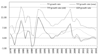
In order to more clearly display the relationship between the changes in GDP growth rate and the changes in total factor input growth rate and total factor productivity growth rate in each year, Figure 1 shows the GDP growth rate curve and the TFI growth rate curve and TFP growth rate curve in China from 1978 to 2019. For comparison, the growth rate curve of total factor productivity for each year calculated using the classical Solow residual method is also plotted. Based on the comparison of the TFP growth rate curves calculated by the two methods in the figure and the data of the capital deepening impact index and the technical progress bias impact index in Table 2, it can be seen that except for the early years of reform and opening up in China, the growth rate of total factor productivity calculated by the new method is basically higher than that calculated by the classical Solow residual method every year. This is because the new growth accounting method constructed under more realistic general technical progress framework successfully decomposes two types of hidden effects: the inhibitory effect of continuous capital deepening on input-output efficiency and the improvement effect of technical progress bias on input-output efficiency. Therefore, the new growth accounting results are closer to reality and more accurate.

Download: Download full-size image

Figure 1. Growrh rats of GDP, TFI and TFP in China.

Download: Download full-size image

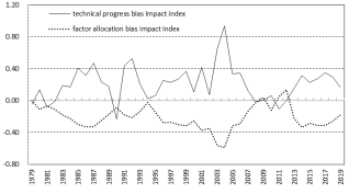
Figure 2. Technical bias impact index and Factor bias impact index.

In order to intuitively reflect the impact of factor allocation bias on economic growth, which is the inhibitory effect of the diminishing marginal returns on factor inputs caused by capital deepening, as well as the counteraction and compensation effects of technical progress bias on input-output efficiency, Figure 2 presents the factor allocation bias impact index and technical progress bias impact index curves for each year from 1978 to 2019 in China. It can be seen that the technical progress bias impact index is almost a mirror image of the factor allocation bias impact index, clearly reflecting the compensation mechanism of technical progress bias for the diminishing marginal returns of factor inputs caused by capital deepening.

Further observation to Figure 2 reveals that since the reform and opening up in China, the impact index of technical progress bias in most years has been greater than the absolute value of the impact index of factor allocation bias in the same year. This indicates that during this period, the bias of technical progress not only compensates for the negative effects of diminishing marginal returns on factor inputs caused by capital deepening, but also has an additional effect on total factor productivity. This additional effect is an important reason why the new growth accounting model calculates a slightly higher total factor productivity growth rate than the classical Solow model.

6. Conclusion

The Hicks neutral technological progress assumption of classical Solow growth accounting does not match the whole reality of economic growth process over the world. This article extends the setting of technical progress to a generalized universal technical progress framework, which can cover various neutral technical progress scenarios such as Hicks neutral, Harrod neutral, and Solow neutral, as well as typical biased technical progress scenarios. Under this general framework of technical progress, the aggregate output index is decomposed into the total factor input index and the total factor productivity index according to the principle of statistical index number. Then, adopting the normalized CES production function with factor augmenting technical progress, and applying the Kmenta’s logarithmic second-order Taylor series expansion of normalized CES production function, the calculation formulas of the total factor input growth rate index and the total factor productivity growth rate index are derived. Thus, a new economic growth accounting system has been established.

The new accounting system not only decomposes the economic growth rate into the sum of the total factor input growth rate and the total factor productivity growth rate, but also further decomposes the two components. The total factor input growth rate is further decomposed into two parts: the factor input intensity growth rate and the factor allocation bias influence rate. The total factor productivity growth rate is also further decomposed into two parts: the technical progress intensity growth rate and the technical progress bias influence rate. The factor allocation bias impact rate reflects the diminishing marginal return effect brought about by capital deepening, while the technical progress bias impact rate is the counteraction and compensation to the diminishing marginal return effect of factor inputs, thus the compensation and counteraction mechanism of technical progress bias to the effect of diminishing marginal return of factor inputs caused by capital deepening is discovered.

The new accounting system covers various scenarios of neutral assumptions in technical progress, as well as various biases scenarios in technical progress. It is applicable not only to mature developed economies that have completed the process of capital deepening and entered a balance growth path, but also to developing economies that are in the stage of sustained capital deepening. The new accounting equation provides a direct calculation method for measuring total factor productivity, rather than relying solely on Solow's "surplus" for indirect calculation. If the elasticity of factor substitution is 1 or there is no bias of technical progress and no bias of factor allocation, then the new accounting equation degenerates into the classical Solow accounting equation, so the Solow accounting equation is a special case of the new accounting equation.

The calculation and decomposition of China's economic growth rate index, total factor input growth rate index, and total factor productivity growth rate index from 1978 to 2019 shows that technical progress bias not only compensates for the negative impact of diminishing marginal returns caused by capital deepening, but also further enhances total factor productivity.

Abbreviations

TRO	Total Real Output
TROG	TRO Growth
TFI	Total Factor Input
TFIG	TFI Growth
TFP	Total Factor Productivity
TFPG	TFP Growth
FII	Factor Input Intensity
FBI	Factor Bias Impact
TPI	Technical Progress Intensity
TBI	Technical Bias Impact

Author Contributions

Lei Qinli is the sole author. The author read and approved the final manuscript.

Conflicts of Interest

The authors declare that they have no conflicts of interest.

References

[1]	Acemoglu D. Directed Technical Change [J]. Review of Economic Studies, 2002, 69(4): 781-810. https://doi.org/10.1111/1467- 937X.00226
[2]	Acemoglu D. Labor- and Capital-Augmenting Technical Change [J]. Joarnal of the European Economic Association. 2003, 1(1): 1-37. https://doi.org/10.1162/154247603322256756
[3]	De La Grandville, Olivier. In Quest of the Slutsky Diamond. [J] The American Economic Review, 1989, 79(3), 468–481. http://www.jstor.org/stable/1806857
[4]	Dong Zhiqing and Chen Rui. Does Total Factor Productivity Growth Result from Biased Technical Change? [J]. Chinese Journal of Management, 2014, 11(8): 1199-1207. https://doi.org/10.3969/j.issn.1672-884x.2014.08.014
[5]	Fei J C H, and Ranis G. Innovational Intensity and Factor Bias in the Theory of Growth [J]. International Economic Review, 1965, 5(2): 182-198. https://doi.org/10.2307/2525414/
[6]	Hao Feng and Sheng Weiyan. Elasticity Estimation of Factor Substitution in China [J]. Statistical Research, 2014, 31(7): 12-21. https://doi.org/10.19343/j.cnki.11-1302/c.2014.07.002
[7]	Klump R, and Grandville O. Economic Growth and the Elasticity of Substitution: Two Theorems and Some Suggestions [J]. The American Economic Review, 2000, 90(1): 282-291. https://doi.org/10.1257/aer.90.1282
[8]	Klump R, McAdam P, and Willman A. Factor Substitution and Factor-augmenting Technical Progress in the United States: A Normalized Supply-side system Approach [J]. Review of Economics and Statistics, 2007, 89(1): 183–192. https://doi.org/10.1162/rest.89.1.183
[9]	Klump R, and Preissler H. CES Production Functions and Economic Growth [J]. The Scandinavian Journal of Economics, 2000, 102(1): 41-56. https://doi.org/10.1111/1467-9442.00183
[10]	Kmenta J. On Estimation of the CES Production Function [J]. International Economic Review, 1967, 8(2): 180-189. https://doi.org/10.2307/2525600
[11]	Lei Qinli. Biased Technical Progress, Capital Efficiency and the Change of Labor Share of Income [J]. Research on Economics and Management, 2012, 33(12): 15-24. https://doi.org/10.13502/j.cnki.issn1000-7636.2012.12.003
[12]	Lei Qinli. The Measure and Analysis of Biased Technical Progress [J]. Statistical Research, 2013, 30(4): 83-91. https://doi.org/10.19343/j.cnki.11-1302.04.014
[13]	Lei Qinli. Institutional Environment and Economic Growth: A Theoretical Model and Empirical Analysis for China [J]. Research on Economic and Management, 2017, 38(12): 3-16. https://doi.org/10.13502/j.cnki.issn1000-7636.2017.12.001
[14]	Lei Qinli and Xu Jiachun. Biased Technological Progress, Biased Factor Allocation, and TFP Growth in China [J]. Statistical Research, 2015, 32(8): 10-16. https://doi.org/10.19343/jcnki.11-1302/c.2015.08.002
[15]	Lei Qinli and Li Yuelin. Capital-Skill Complementarity and the Direction of skill Bias of Technological Progress [J]. Statistical Research, 2020, 37(3): 48-59. https://doi.org/10.19343/jcnki.11-1302 /e.2020.03.004
[16]	Leon-ledesma M, McAdam P, and Willman A. Identifying the Elasticity of Substitution with Biased Technical Change [J]. American Economic Review, 2010. 100(4).1330-1357. https://doi.org/10.1257/aer.100.4.1330
[17]	Leon-ledesma M, McAdam P, and Willman A. Production Technology Estimates and Balanced Growth [J]. Oxford Bulletin of Economics and Statistics, 2015, 77(1): 40-65. https://doi.org/10.1111/obes.12049
[18]	OECD. Measuring Productivity - OECD Manual: Measurement of Aggregate and Industry-level Productivity Growth,[M] OECD Publishing, 16 Jul 2001, Paris, https://doi.org/10.1787/9789264194519-en
[19]	Papageorgiou C. and Saam M. Two-level CES Production Technology in the Solow and Diamond Growth Models [J]. Scandinavian Journal of Economics, 2008. 110(1), 119-143. https://doi.org/10.1111/j.1467-9442.2008.00529.x
[20]	Solow R M. Technical Change and the Aggregate Production Function [J]. The Review of Economics and Statistics, 1957, 39(8): 312-320. https://doi.org/10.2307/1926047
[21]	Yu Donghua and Chen Ruying. Capital Deepening, Factor Income Share and Total Factor Productivity— A Perspective from Biased Technical Change. Journal of Shandong University (Philosophy and Social Sciences), 2020(5): 107-117. https://doi.org/10.19836/j.cnki.37-1100/c.2020.05.011

Cite This Article

Plain Text BibTeX RIS

APA Style

Qinli, L. (2024). Measuring Total Factor Productivity in General Technical Progress Framework. American Journal of Theoretical and Applied Statistics, 13(6), 181-192. https://doi.org/10.11648/j.ajtas.20241306.11

Copy | Download

ACS Style

Qinli, L. Measuring Total Factor Productivity in General Technical Progress Framework. Am. J. Theor. Appl. Stat. 2024, 13(6), 181-192. doi: 10.11648/j.ajtas.20241306.11

Copy | Download

AMA Style

Qinli L. Measuring Total Factor Productivity in General Technical Progress Framework. Am J Theor Appl Stat. 2024;13(6):181-192. doi: 10.11648/j.ajtas.20241306.11

Copy | Download

@article{10.11648/j.ajtas.20241306.11,
  author = {Lei Qinli},
  title = {Measuring Total Factor Productivity in General Technical Progress Framework
},
  journal = {American Journal of Theoretical and Applied Statistics},
  volume = {13},
  number = {6},
  pages = {181-192},
  doi = {10.11648/j.ajtas.20241306.11},
  url = {https://doi.org/10.11648/j.ajtas.20241306.11},
  eprint = {https://article.sciencepublishinggroup.com/pdf/10.11648.j.ajtas.20241306.11},
  abstract = {The classical Solow's total factor productivity accounting assumes that technical progress is Hicks neutral, which is a special situation in the reality of world economy. This paper expands the setting of technical progress into general technical progress framework, which can cover Hicks neutral technical progress, Harrod neutral technical progress, Solow-neutral technical progress, and various factor-biased technical changes. According to the principle of statistical index number, this paper decomposes the output index into a total factor input index and a total factor productivity index, and adopts normalized CES production function with factor-augmenting technical progress to derive the calculation formulas of the total factor input index and the total factor productivity index, and constructs a new economic growth accounting system, and finds the counteraction and compensation mechanism for diminishing marginal returns. If the factor substitution elasticity is 1 or there is no technical progress bias and factor allocation bias, then the new accounting equation degenerates into the classic Solow growth accounting equation. The new accounting system can measure the influence of total factor input and total factor productivity to economic growth, but also can measure the influences of factor input intensity and factor allocation bias in the growth rate of total factor input, and the influences of technical progress intensity and technical progress bias in the growth rate of total factor productivity. Therefore it is more precise and accurate than classical method.
},
 year = {2024}
}

Copy | Download

TY  - JOUR
T1  - Measuring Total Factor Productivity in General Technical Progress Framework

AU  - Lei Qinli
Y1  - 2024/11/12
PY  - 2024
N1  - https://doi.org/10.11648/j.ajtas.20241306.11
DO  - 10.11648/j.ajtas.20241306.11
T2  - American Journal of Theoretical and Applied Statistics
JF  - American Journal of Theoretical and Applied Statistics
JO  - American Journal of Theoretical and Applied Statistics
SP  - 181
EP  - 192
PB  - Science Publishing Group
SN  - 2326-9006
UR  - https://doi.org/10.11648/j.ajtas.20241306.11
AB  - The classical Solow's total factor productivity accounting assumes that technical progress is Hicks neutral, which is a special situation in the reality of world economy. This paper expands the setting of technical progress into general technical progress framework, which can cover Hicks neutral technical progress, Harrod neutral technical progress, Solow-neutral technical progress, and various factor-biased technical changes. According to the principle of statistical index number, this paper decomposes the output index into a total factor input index and a total factor productivity index, and adopts normalized CES production function with factor-augmenting technical progress to derive the calculation formulas of the total factor input index and the total factor productivity index, and constructs a new economic growth accounting system, and finds the counteraction and compensation mechanism for diminishing marginal returns. If the factor substitution elasticity is 1 or there is no technical progress bias and factor allocation bias, then the new accounting equation degenerates into the classic Solow growth accounting equation. The new accounting system can measure the influence of total factor input and total factor productivity to economic growth, but also can measure the influences of factor input intensity and factor allocation bias in the growth rate of total factor input, and the influences of technical progress intensity and technical progress bias in the growth rate of total factor productivity. Therefore it is more precise and accurate than classical method.

VL  - 13
IS  - 6
ER  -

Copy | Download

Author Information

Lei Qinli

Department of Economic Statistics, Guangzhou Huashang College, Guangzhou, China

Contact Email

Download PDF

Submit an Article

Plain Text BibTeX RIS

APA Style

Qinli, L. (2024). Measuring Total Factor Productivity in General Technical Progress Framework. American Journal of Theoretical and Applied Statistics, 13(6), 181-192. https://doi.org/10.11648/j.ajtas.20241306.11

Copy | Download

ACS Style

Qinli, L. Measuring Total Factor Productivity in General Technical Progress Framework. Am. J. Theor. Appl. Stat. 2024, 13(6), 181-192. doi: 10.11648/j.ajtas.20241306.11

Copy | Download

AMA Style

Qinli L. Measuring Total Factor Productivity in General Technical Progress Framework. Am J Theor Appl Stat. 2024;13(6):181-192. doi: 10.11648/j.ajtas.20241306.11

Copy | Download

@article{10.11648/j.ajtas.20241306.11,
  author = {Lei Qinli},
  title = {Measuring Total Factor Productivity in General Technical Progress Framework
},
  journal = {American Journal of Theoretical and Applied Statistics},
  volume = {13},
  number = {6},
  pages = {181-192},
  doi = {10.11648/j.ajtas.20241306.11},
  url = {https://doi.org/10.11648/j.ajtas.20241306.11},
  eprint = {https://article.sciencepublishinggroup.com/pdf/10.11648.j.ajtas.20241306.11},
  abstract = {The classical Solow's total factor productivity accounting assumes that technical progress is Hicks neutral, which is a special situation in the reality of world economy. This paper expands the setting of technical progress into general technical progress framework, which can cover Hicks neutral technical progress, Harrod neutral technical progress, Solow-neutral technical progress, and various factor-biased technical changes. According to the principle of statistical index number, this paper decomposes the output index into a total factor input index and a total factor productivity index, and adopts normalized CES production function with factor-augmenting technical progress to derive the calculation formulas of the total factor input index and the total factor productivity index, and constructs a new economic growth accounting system, and finds the counteraction and compensation mechanism for diminishing marginal returns. If the factor substitution elasticity is 1 or there is no technical progress bias and factor allocation bias, then the new accounting equation degenerates into the classic Solow growth accounting equation. The new accounting system can measure the influence of total factor input and total factor productivity to economic growth, but also can measure the influences of factor input intensity and factor allocation bias in the growth rate of total factor input, and the influences of technical progress intensity and technical progress bias in the growth rate of total factor productivity. Therefore it is more precise and accurate than classical method.
},
 year = {2024}
}

Copy | Download

TY  - JOUR
T1  - Measuring Total Factor Productivity in General Technical Progress Framework

AU  - Lei Qinli
Y1  - 2024/11/12
PY  - 2024
N1  - https://doi.org/10.11648/j.ajtas.20241306.11
DO  - 10.11648/j.ajtas.20241306.11
T2  - American Journal of Theoretical and Applied Statistics
JF  - American Journal of Theoretical and Applied Statistics
JO  - American Journal of Theoretical and Applied Statistics
SP  - 181
EP  - 192
PB  - Science Publishing Group
SN  - 2326-9006
UR  - https://doi.org/10.11648/j.ajtas.20241306.11
AB  - The classical Solow's total factor productivity accounting assumes that technical progress is Hicks neutral, which is a special situation in the reality of world economy. This paper expands the setting of technical progress into general technical progress framework, which can cover Hicks neutral technical progress, Harrod neutral technical progress, Solow-neutral technical progress, and various factor-biased technical changes. According to the principle of statistical index number, this paper decomposes the output index into a total factor input index and a total factor productivity index, and adopts normalized CES production function with factor-augmenting technical progress to derive the calculation formulas of the total factor input index and the total factor productivity index, and constructs a new economic growth accounting system, and finds the counteraction and compensation mechanism for diminishing marginal returns. If the factor substitution elasticity is 1 or there is no technical progress bias and factor allocation bias, then the new accounting equation degenerates into the classic Solow growth accounting equation. The new accounting system can measure the influence of total factor input and total factor productivity to economic growth, but also can measure the influences of factor input intensity and factor allocation bias in the growth rate of total factor input, and the influences of technical progress intensity and technical progress bias in the growth rate of total factor productivity. Therefore it is more precise and accurate than classical method.

VL  - 13
IS  - 6
ER  -

Copy | Download