Research Article | | Peer-Reviewed

Impact of Changes in Fuel Prices on Inflation and Economic Growth in Mozambique

Received: 21 April 2024    Accepted: 13 May 2024    Published: 30 May 2024
Views:       Downloads:
Abstract

The fuel oil is a basic input to production, so an increase in oil price leads to a rise in production costs that induces firms to lower output. In parallel, oil prices change also effects, indirectly, the consumption, through its positive relation with disposable income. However, despite the relevance of the variation in fuel prices in economy, there are no recent study conducted to analyse the impact of changes in fuel prices on GDP and CPI in Mozambique. This study aims to contribute to filling the information gap by providing the quantification of the impact of fuel prices on GDP and CPI. So, the study aim to determine the impact of changes in FUEL prices on Inflation (Consumer Price Index – CPI) and Economic Growth (Gross Domestic Product – GDP), using quarter data from 2007 to 2020. Descriptive statistics, Unit Root Test, Johansen Cointegration Test and Error Correction Model, Granger Causality Econometric Models, Impulse and Response Function and Variance Decomposition Analysis are used. The results indicate that in Mozambique there are a cointegrating long-run relationship between FUEL prices and CPI and GDP, which suggest that the impact of FUEL prices shocks to CPI and GDP in short-run and long-run path. Also, the results show that changes in GDP and FUEL prices lead to an increase in CPI by 3.0% and 1.3%, respectively, coeteris paribus. The previous quarter’s errors (or deviation from long-run equilibrium) are corrected for with the current quarter at a convergence speed of 3.5% to GDP, and 4.8% to CPI. Granger causality tests also indicate causality between CPI and GDP, and the changes in GDP causes changes in other variables.

Published in International Journal of Economics, Finance and Management Sciences (Volume 12, Issue 3)
DOI 10.11648/j.ijefm.20241203.12
Page(s) 142-160
Creative Commons

This is an Open Access article, distributed under the terms of the Creative Commons Attribution 4.0 International License (http://creativecommons.org/licenses/by/4.0/), which permits unrestricted use, distribution and reproduction in any medium or format, provided the original work is properly cited.

Copyright

Copyright © The Author(s), 2024. Published by Science Publishing Group

Keywords

FUEL, Consumer Price Index, Gross Domestic Product, Vector Autoregressive, Vector Error Correction Model

1. Introduction
The fuel oil plays an important role in various productive activities. So, when the oil prices increases, the production costs increases too, which induces firms to lower output. In parallel, oil prices change also effects, indirectly, the consumption, through its positive relation with disposable income. Moreover, oil prices have an adverse impact on investment by increasing firms’ costs, and, also influence foreign exchange markets and inflation .
In various parts of the world, and over time, several studies have been conducted to assess the impact of oil shocks on the economy . Most of these authors indicates that there are a positive relationship between oil price and the rate of inflation whereas an inverse relation exists between oil price and economic growth.
The inflation of fuel and food prices worldwide represents a negative terms-of-trade shock for Mozambique because the country is fuel importer . The rising prices of food and fuel, associated with others factors, - such poverty, unemployment, and social injustice-, are precipating conditions for social unrest. . On other hands, other authors argue that increasing of fuel prices are in most cases an suggestion of an imminent recession .
However, despite the relevance of the variation in fuel prices in economy, there are no recent study conducted to analyze the influence of changes in fuel prices on GDP and CPI in Mozambique. This study wishes to contribute to filling the information gap by providing the quantification of the impact of fuel prices on Gross Domestic Product (GDP) and Consumer Price Index (CPI). The overall objective of this study is to determine the magnitude of the impact of changes in the fuel price on macro-economic variables such GDP and CPI.
2. Literature Review
This chapter reviews the literature and is divided into two subchapters. Subchapter 2.1 deals with the theoretical aspects of GDP and CPI and subchapter 2.2 is reserved for reviewing the empirical literature on the impact of fuel prices on inflation and GDP in various parts of the world.
2.1. Gross Domestic Product and Consumer Prices Index in Mozambique
For the United States Department of Commerce the Gross Domestic Product (GDP) is one of the great inventions of the 20th century and a powerful statistic in the history of humanity and three people played a key role in the history of GDP, Petty, Clark and Kuznets, Therefore, the idea of calculating a national income dates back to the 17th century with the initiatives of William Petty (1623-1687) in England, passing through the works of Colin Clark (1905-1989), also in England, who formulated many of the updated elements in the pattern of GDP compilation, until culminating with the work carried out by the team led by Simon Kuznets (1901-1985) in the United States .
The Gross Domestic Product (GDP) is the sum of gross value added of all resident producer units plus that part (possibly the total) of taxes on products, less subsidies on products, that is not included in the valuation of output. GDP is also equal to the sum of the final uses of goods and services (all uses except intermediate consumption) measured at purchasers’ prices, less the value of imports of goods and services. Finally, GDP is also equal to the sum of primary incomes distributed by resident producer units .
The conceptual reference of the general compilation framework of National Accounts in Mozambique is the 2008 System of National Accounts (SNA 2008) developed by the United Nations (UN) in partnership with the International Monetary Fund (IMF), the European Union (EU), the World Bank (WB) and the Organization for Economic Co-operation and Development (OECD). The United Nations Statistics Division (UNSD) Compilation Manual “A System Approach to National Accounting Compilation” is followed to process the information, which presents a practical structure for compiling a country's national accounts.
The figure 1 shows that the Mozambican economy is dominated by the primary sector (agriculture, livestock, forestry, fishing and extractive industry), with a stable weight of more than a third of GDP and second place are the various services including public administration with about a quarter of GDP. On the other hand, services from transport and communications activities, which are directly impacted by the rise in fuel prices, represent around 5% of GDP and the industry about 12%.
The low preponderance of transport services is the fact that 67% of the population of Mozambique live in rural areas and practice agriculture, livestock, fishing, mineral extraction, in a rudimentary way, without access to credit and with little use of machiner may justify a possible residual impact of rising fuel prices on economic growth.
Consumer Price Index (CPI) is an index that measures the rate at which the prices of consumption goods and services are changing from one period to another and is widely used as a proxy measure of inflation for the economy as a whole (21). The usual method of calculation is to take an average of the period-to-period price changes for the different products, using as weights the average amounts that households spend on them. CPIs are official statistics that are usually produced by National Statistical Office, ministries of labour, or central banks.
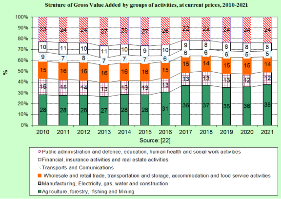
Figure 1. Structure of Gross Value Added by activity groups at current prices, 2010-2021.
Since 1997, Mozambique National Institute of Statistics is the entity responsible for the compilation and official dissemination of the CPI. The first consistent series of indices had the month of December 1994 as its base period and was limited only to the City of Maputo and was taken as a reference for the National CPI. Following international recommendations, the CPI weights are derived based on the results of the representative survey that the Household Budget Survey . The classification used is the Classification of Individual Consumption by Purpose (COICOP). The table below shows the evolution of the CPI weights by division of COICOP, where the division of food and non-alcoholic beverages is preeminent with the highest weights, and that is determinant of inflation in Mozambique.
Table 1. Evolution of the CPI weight by division of COICOP.

Division Code

Description

Base: Dez.98

Base: Dez.2004

Base: Dez.2010

Base: 2016=100

01

Food and non-alcoholic beverages

62,4

55,46

44,48

33,92

02

Alcoholic beverages, tobacco and narcotics

1,06

2,21

1,32

1,21

03

Clothing and footwear

4,62

4,65

8,45

7,4

04

Housing, water, electricity, gas and other fuels

12,17

12,62

12,9

7,36

05

Furnishings, household equipment and routine household maintenance

4,79

5,3

6,37

7,59

06

Health

2,46

2,94

1,45

0,88

07

Transport

2,83

7,92

11,67

17,06

08

Information and communication

1,8

1,72

3,37

6,36

09

Recreation, sport and culture

2,12

2,63

3,52

1,57

10

Education services

0,63

1,26

1,71

2,38

11

Restaurants and accommodation services

0,34

1,97

1,34

10,7

12

Other Goods and Services

4,78

1,32

3,42

3,57

Total

100

100

100

100

Source:
In contrast to the structure of GDP, where transport services have a low weight, deducing from this a possible residual effect of changes in fuel prices on GDP, when analyzing the weights of the CPI in table 1, it is noted that transport services has a relevant weight, ranking second with 17.06%, right after food products, which have 33.92%. Thus, it is to be expected that any variation in fuel prices will have a significant effect on inflation.
2.2. Empirical Review of Influence of Variations in Fuel Prices to Inflation and Economic Growth
Many studies were carried out in different countries and at different times, and the results suggest that the increase in fuel prices has an economic and social impact. The rise in the price of petroleum products is passed from the consumer standpoint (households, industry and government), the energy bill grows, whereas from the production standpoint, companies have to contend with a rise in unit costs. The increase of fuel prices causes a drop-in productivity, which is passed on to (i) real wages and employment; (ii) selling prices and core inflation; (iii) profits and investment, as well as stock market capitalization .
Among the numerous impacts of the increase in fuel prices, can be highlighted the following: (i) socio-economic unrest which result in increase in transport fare; (ii) inflation in both public and private life with a consequent increase in prices of goods and services; (iii) corruption by both government and private individual, discourages foreign direct investment; (iv) complication in economic growth, because of its negative impact on the socio-economic life of the people; (v) importation cost of fuel that leads to huge and excessive public expenditure on importation of fuel to augment local production which in itself is an indication of an unhealthy economy resulting in accumulated balance of payments deficit .
Several authors have used time series econometrics for the investigation the effect of fuel prices on CPI. Mainly the Vector Auto regression (VAR) model and Vector Error Correction Model (VECM) are used, since they are among the most successful, flexible, and easy to use models. Most of them have indicated that growing fuel prices have a positive influence on inflation . On the same line, other authors studied the impact of fuel prices on GDP and CPI and, as a general rule, show that the increase in fuel prices is associated with a reduction in GDP . However, other studies concluded that the rise in fuel prices causes an increase in GDP .
The study of the impact of oil price variation on the rate of inflation in two groups of countries, namely the high versus low oil dependency groups, detected long-run relationship between oil price changes and inflation . The changes of oil price have significance effects on determining the domestic inflation. Also, the results showed that fuel oil price change has its direct consequence on domestic inflation in low oil dependency group but its impact is indirect on determining the domestic inflation in high oil dependency group.
The results also showed that the main determinants of domestic inflation are real exchange rate and exporter’s production cost (high oil dependency group) and domestic output and exporter’s production cost (low oil dependency group) . The authors suggest the policymaker to concern on the effects of oil price, real exchange rate and exporter’s production cost on domestic inflation as they are important factors that can affect the stability of prices and financial variable estimated coefficient high oil dependency low oil dependency long-run parameter .
In Turkey was analyzed the long-term inflationary effect of price of oil products and their results indicate that a 10% increase in the price of oil products increases the inflation in a rate of 4.52% . Inflationary effects of price increases of oil products, more than the import price, appear to have emerged particularly depending on the pricing in the national market . The inflationary effect of oil products, although were significant and positive as in the long term, were rather in a small value in the short-term analysis.
Also, was investigated the effects of changes of the oil price on inflation for the G-5 countries (United States, United Kingdom, France, Germany and Japan) and the results depicted that the oil price increase is likely to have only a modest effect on inflation in the United States, Japan and Europe . Oil price increase as much as 10 percentage points will lead to a direct inflationary increase of about 0.1–0.8 percentage points in the United States and the European Union.
Inflation in Europe, traditionally thought to be more sensitive to oil prices than in the United States, is unlikely to show any significant difference in sensitivity to that in the United States and in fact may be less in some countries. The statistical estimates suggest that oil price increases are likely to have only a modest effect on inflation in the U.S, Japan, and Europe.
The analysis of the impact of oil prices on inflation and industrial production indexes for many European countries using quarterly data for the period 1960–1999, indicate that the oil prices have permanent effects on inflation and short run but asymmetric effects on production growth rates . There is not a cointegrating long-run relationship between oil prices and economic activity, which suggest that the impact of oil shocks on these variables is limited to the short-run .
When analyzing short-run relationship between oil prices and economic growth rates, oil prices shocks was found to Granger cause economic growth rates, in Japan, South Korea and Thailand (in the last case, only when oil prices are defined in local currency) when several non-linear specifications are used to model the relationship between the variables. Also, was found evidence of asymmetries in the oil prices changes-inflation rate relationship for the case of Japan, Thailand, South Korea and Malaysia, and only for the case of South Korea when the oil prices changes-economic growth rate relationship is analyzed .
Studies conducted to assess the impact of fuel on the Nigerian economy have concluded that there exists a direct relationship between fuel price increase and the inflation rate in Nigeria and whenever petroleum increases, the inflation rate also increases .
The analysis of the impact of increased oil prices in the Nigerian economy based upon the annual data from 1990 to 2011, concluded that the petroleum products like gasoline and automotive gas oil have a positive relationship with the level of the inflation rate . According the results of this study a unit change in gasoline has the potential to induce about 50.324 percentage change in the response of inflation rate in the same direction. Similarly, one percentage change in automotive gas oil has the potential to induce about 9.702 percentage change in the response of inflation also in the same direction. The Error Correction Mechanism from the study was (-0.717) implying that inflation rate will adjust to change in petroleum products in the short-run at the rate of 72 percent.
Also in Nigeria, was studied the effect of petroleum product prices adjustment on inflation rate during 1980-2021, and the results showed that a 1% increase in the prices of gasoline and automotive gas oil increased inflation rate by 0.074 and 0.022 respectively . The Error Correction Mechanism exhibited the hypothesized negative sign (– 0.400065) implying that the speed of adjustment to long run steady state is about 40 per cent and importantly, it is statistically significant at 5 per cent level .
The study about the relationship between oil price shocks and China’s macroeconomy using the monthly time series data from 1995:1 to 2008:12, showed that changes in the world oil prices have a significant effect on the inflation and the economic growth in China and the impact is non-linear . The impulse-response functions of the linear impact model show that China’s GDP and CPI are both positively correlated with the world oil price, the largest impact reaches in the second month and disappears completely after about 12 months. As an oil importing country, an increase in oil price should have increased the production costs of China, and thus retarded its GDP growth, but this does not appear to be happening. The impulse-response functions of the linear impact model show that China’s GDP and CPI are both positively correlated with the world oil price, the largest impact reaches in the second month and disappears completely after about 12 months . Cumulatively, a 100% increase of the world oil price increases GDP and CPI of China by about 9% and 2.08, respectively.
The results of non-linear models show that the impact of the world oil price on China’s GDP is asymmetric. The impact of the positive oil price shocks is not significant, while the negative oil price shocks decrease the economic growth of China significantly, though the magnitudes of the impact of the three non-linear models are different .
Similarly, analysed the impact of crude oil price on the rate of inflation and economic growth in India. The results showed that the crude oil price has a positive impact on the rate of inflation whereas an inverse relation exists between crude oil price and economic growth . The empirical results derived from structural VAR framework observed that oil price has a positive impact on inflation rate whereas an inverse relation exists between oil price and economic growth. More specifically, 1% fall in oil price leads to 0.49% fall in the inflation rate in India over the period and vice versa; and 1% fall in oil price leads to a rise of 0.81% in economic growth, and vice versa.
Also, in India, was analyzed the impact of increase in oil prices on inflation and output, and the results showed that a 20% shock in oil prices leads to a 1.3% increase in inflation of the other commodities and a reduction in the output growth by 2.1 . The impulse response functions from the VAR model revealed that a 20-percentage point shock in oil prices lead to a 1.3 percentage point increase in inflation in other commodities at its peak, which typically occurred after five to seven months after the shock. The impact on prices persists for about two years, though during the later period it lessens considerably in magnitude. In response to a shock of similar magnitude, growth in output decelerates by about 2.1 percentage point and recovery starts to take place approximately after a year .
For the Kenyan reality, was studied the effects of crude oil prices on gross domestic product growth and selected macroeconomic variables using three Autoregressive Distributed lag (ARDL) . The findings of the study revealed that, in Kenia crude oil prices have a positive long-run effect on GDP growth and inflation, while in the short run its lag of one has the effect on inflation rate, meaning that the crude oil prices for the previous one year affects the current year’s inflation. If crude oil price increases by $1, GDP will increase by 0.016 percent in the long run. The long run coefficient of crude oil prices shows that when crude oil prices increases by $1, this would lead to an increase in inflation rate by 0.049 percent in the long run. The study also established that in the short run, a rise in crude oil price by $1 in the previous year, would result to a rise in inflation rate in the current year by 0.114 percent .
Likewise, was analyzed the effect of changes of fuel price on industrialized countries from 1986 to 2010 and their results reveals that rising fuel prices reduce the growth of GDP and an increase in inflation . The study concluded that, in particular, all net oil and energy importing countries are confronted with a permanent fall in economic activity and a rise of inflation. On the other hand, the long-run impact on real GDP is insignificant or even positive in countries that are net energy-exporters. Also, the results show that the change in the economic effects should be more favorable for countries that improved their oil and energy position the most over time, and the degree of improvement in oil and energy dependence is indeed important for time-variation in the effects of oil supply shocks and oil-specific demand shocks and for explaining the associated cross-country differences .
In Russia was analyzed the fuel exporting and fuel importing countries regarding the influence of changes in fuel price on GDP and found that, a fuel exporting country, fuel price increases positively supported GDP growth . On the other hand, for countries such as Japan, US, China, Finland, Germany and the UK, fuel price increase had a negative impact on GDP. The authors conclude that Russia, as a net oil exporter, gains from oil price shocks in both the short and long run. Moreover, the positive effect is quite large, indicating that a 50% increase in the positive oil price growth rate in the current quarter leads to 12.6 and 8.52 percentage point increases in cumulative GDP after 4 and 20 quarters .
Furthermore, was analyzed the effect of fuel prices on macro-economic variables in 36 countries which included fuel importing and exporting countries . In long-run relationships were found that rising in fuel price have a negative influence on GDP, while on the short-run, Granger causality indicated that causality runs from fuel prices to other variables. The authors found that fuel price shocks do not have a significant impact on other macro-economic variables in Nigeria. The results, also show that the impact of an increase in oil prices is always negative. For instance, in Italy, a 10% oil price increase leads to a - 0.7% decrease in GDP. It should be noted that oil prices also have a large impact on unemployment rates for these countries, the impact being globally negative. A 10% increase in oil prices leads to a 3.7% decrease in UK share prices and 4.5% for Malaysia.
In South Africa was analyzed the effect of variations in the fuel price on inflation and economic growth by means of the Johansen cointegration and Granger causality econometric models, and the results indicated both long and short-run relationships between the variables . In the long-run, with inflation as the dependent variable, fuel and GDP both have significant and positive relationships with the dependent variable. So, an growth in the fuel price level have an increasing impact on inflation, such, a one percent increase in the fuel price induces a 0.15 percent increase in inflation, while an increase in GDP growth leads to an even higher impact on inflation. Considering the GDP as the dependent variable, the fuel price has a negative impact on GDP while an increase in inflation as a positive impact on GDP on the long run. The results also reveals that the GDP has a short-run relationship with inflation, therefore, 1.4 percent of the disequilibrium in GDP is corrected in each quarter. Further short-run results indicate that fuel has a positive significant impact on inflation; GDP has a positive impact on fuel; changes in inflation has a negative impact on GDP; and change in fuel leads to reduction of GDP .
Other authors concluded that the results obtained from vector autoregressions are broadly consistent with the expectation that the real GDP growth of oil importing economies suffers from increases in oil prices in both linear and non-linear models . With regard to the two net oil exporters, Norway benefits from oil price hikes while in the UK a rise in oil prices is found to have a significant negative impact on GDP growth. These contrasting results for oil exporting countries can be traced to a sharper real exchange-rate appreciation in the case of the UK. In the case of net oil importer Japan, the results obtained using the optimal order of the model (i.e. four lags) indicate a positive association between oil prices and real performance. This unexpected result can be rationalized in terms of the peculiar circumstances undergone by the Japanese economy during the period under study. Furthermore, the unexpected result is not robust, being reversed in the case of a second-order vector autoregression .
3. Methodology
The study focuses on Mozambique as a fuel importing country, and analyze the impact of changes in the fuel price on GDP and CPI. The study follows a quantitative approach based on a dataset of 59 quarterly observations from quarter one of 2007 to quarter three of 2021. The period was choice due to availability of data. Variables included in the study are the monthly data of price of fuel in Mozambique currency (MZM).
In this study, fuel prices correspond to average prices of gasoline and diesel, which are the most consumed types of liquid fuels in Mozambique, representing more than 90% of fuel imports (INE, 2022); quarter GDP at constant prices and monthly data of CPI. The data was derived from National Statistics Institute (INE- Instituto Nacional de Estatística, in Portuguese). To ensure uniformity, CPI and fuel prices data were quarterly. On the other hand, there was a need for chaining retropolation CPI data, since the original data cover series periods of bases not yet linked. The Lisman and Sandee method was used to transform the annual GDP to quarter). To a certain extent the Lisman and Sandee method contains some arbitrary aspects, but it has the advantage of simplicity, plausibility and practical usefulness .
The main objective of the study was to determine the impact of fuel price changes on economic activity, measured as GDP and also on the CPI rate in Mozambique. Thus, in the study to analyze the impact of fuel prices on the South African economy, the following equations are used as to achieve the objective :
LNCPI = f (LNFUEL,LNGDP)(1)
Where: LNCPI is the natural logarithm of the CPI, LNGDP is the natural logarithm of real Gross Domestic Product (GDP) and LNFUEL is the natural logarithm of the fuel price in MZM. All variables were converted to their natural logarithms for the adjustment of any likelihood of scale effect and to estimate growth or elasticities.
3.1. Cointegration Procedure
The study employs three techniques to analyze the study objectives: (1) the Johansen cointegration technique within the vector autoregressive (VAR) model, (2) the Vector Error Correction Mechanism (VECM) and (3) the Impulse Response Function (IRF). The Johansen cointegration test, which explores cointegration, is used to express the dynamic relationship amongst the variables of interest, and to observe the short- and long-run dynamics of the model.
Evidence from most studies suggests that many economic time series are nom-stationary (integrated of order one or higher). Yet, it is possible that some combination of time series may drift together, at least in the long-run.
The intuition here is that for the two variables to form a meaningful long-run relationship, they must share a common stochastic trend in the long-run. That is, there may exist some linear combination of the variable that, over time, converge to an equilibrium. Otherwise, they would be drifting away from each other over time. Therefore, to build econometric models which makes sense in the long-run, we have to test if the variables are integrated and if they form cointegrating relationship. However, if all variables are found to be non-stationary then a cointegration test is estimated to determine whether a linear combination of such non-stationary variables is stationary.
Prior to conducting the analysis, the Augmented Dickey-Fuller (ADF) test was used to test the variables for stationarity or unit root. If the observed variables are found to be stationary, then the VAR model in equation (1) was estimated. To make sure that the regression is not spurious, the unit root properties of variables were first examined with the Dickey and Fuller (ADF). The augmented Dickey-Fuller (ADF) unit root test is specified as follows .
(2)
where is a pure white noise error term and where , , etc. The number of lagged difference terms to include is often determined empirically, the idea being to include enough terms so that the error term is serially uncorrelated. In ADF we still test whether δ = 0 and the ADF test follows the same asymptotic distribution as the DF statistic, so the same critical values can be used.
Cointegration can be tested in two ways the first involves testing the null hypothesis that residuals from cointegration regression has a unit root against the alternative that the residual series is stationary. The system-based cointegration procedure developed by Johansen and Juselius in 1990 to test the absence or presence of long run equilibrium is adopted in this paper .
The Johansen method commences from a standard Vector Autoregressive (VAR) of the form.
𝑋𝑡1𝑋𝑡+...+Π𝑘𝑋𝑡−𝑘+𝜇+𝐷𝑖+𝑖(3)
Where X is a Px1vector of the I(1) variable of interest, 𝜇is a vector of constant, D is a vector of centered seasonal dummies and 𝑖are IN (0, Δ) error term.
Letting Δ represents the first difference operator, is suggested to be writing the precede equation in the equivalent form as :
Δ𝑋𝑡=Γ𝑖Δ𝑋𝑡−1+...+Γ𝑘−1Δ𝑋𝑡−𝑘−1 +Π𝑥𝑡−𝑘+𝜇+𝐷𝑖+𝑡
Γ𝑖= −𝐼+Π1+...+Π(𝐼=1,...,𝑘−1)𝑎𝑛𝑑Π= −𝐼+Π1+...+Π𝑘(4)
The equation of stationary error-first difference VAR where the term Π𝑥𝑡−𝑘, contains information on the long-run (levels) relationships between the variable in the VAR . Cointegration can be detected by examining the Π matrix. If the pxp matrix Π has rank 0, then all elements of Xt have unit root and first-differencing might be recommended. There are three possible cases:
1. Rank (Π) = p, i.e, the matrix Π has full rank, indicating that the vector process Xt is stationary (all elements are stationary in levels).
2. Rank (Π) = 0, i.e, the matrix Π is the null matrix and the equation corresponds to a traditional differenced vector time series model.
3. 0<rank<(Π) = r<p. implying that there are pxr matrices 𝛼and 𝛽 such that Π = 𝛼𝛽′. In this case, it is said that there are cointegrating relations among the elements of Xt, and (p-r) are common stochastic trends. If Π has rank r<p, this implies that
Π=𝛼𝛽′(5)
Where 𝛼and 𝛽are VxP, with 𝛽 containing the V cointegrating vectors, and 𝛼their corresponding.
The existence of cointegrating relationships between the variables further implies undertaking the Vector Error Correction Model (VECM) . Alternatively, the study may proceed with the VAR model of the first differenced in case there are no co-integrating relationships.
The VECM is a cointegrated VAR, which is only justified and important after establishing the existence of a long-run relationship among the variables. This gives the instance to evaluate the cointegrated series. The conventional multivariate VECM is written compactly as follows:
(6)
where yt is as explained previously; X’ is the vector of endogenous regressors; ECTt-1 is the lagged Ordinary Least Square (OLS) residual obtained from the long-run cointegrating equation given as 𝐸𝐶𝑇𝑡−1 = 𝑌𝑡−1 1𝑋𝑡−1 the cointegrating equation, which deviates from the previous period from the long-run equilibrium (which is an error), affects the short-run movement in the dependent variable; λ is the coefficient of the ECT and the speed of adjustment, which measures the speed at which y returns to equilibrium after changes in X’; γ, η are parameters to be estimated; k is the optimal lag length and ut is the white-noise error.
VECM is a special case of VAR that imposes cointegration on its variables where it allows us to distinguish between short run and long run Granger causality. The relevant Error Correction Terms (ECTs) must be included in the VAR to avoid misspecification and omission of the important constraints. The existence of a cointegrated relationship in the long run indicates that the residuals from the cointegration equation can be formulated as follows :
ΔGDP=α0+i=1mβ1.iΔGDPt-1+i=1nβ2.iFUELt-1+i=1oβ3.iCPIt-1+μ1ECTt-1+1tΔFUEL=δ0+i=1mφ1.iΔGDPt-1+i=1nφ2.iFUELt-1+o=1iφ3.iCPIt-1+μ2ECTt-1+2tΔCPI=σ0+i=1mϕ1.iΔGDPt-1+i=1nϕ2.iFUELt-1+i=1oϕ3.iCPIt-1+μ3ECTt-1+3t(7)
where is the lag operator, 𝛼0, 𝛿0, 𝜎0; are the estimated coefficients. 𝛽' s, 𝜙′𝑠 and 𝜑's are short-run dynamic coefficients of the model’s adjustment long-run equilibrium. The m and n are the optimal lags of the series GDP, CPI and FUEL, reduced by 1; ’s are the serially uncorrelated error terms; while 𝜇1 and 𝜇2 𝜇3 represents the speed of adjustment parameter with a negative sign, measure a single period response of the GDP, CPI and FUEL to a departure from equilibrium. 𝐸𝐶𝑇𝑡−1 is the Error Correction Term and represents the lagged value of the residuals obtained from the cointegrating regression of the dependent variable on the regressors. The ECT contains long-run information derived from the long run cointegrating relationship.
3.2. Impulse Response Function
There are numerous interesting applications, in which a researcher might be interested in calculating an impulse response function. Without any loss of consistency, this approach accommodates interactions among the variables in the system. A further advantage of the IRF is that it can also be used to evaluate the effect of a policy change on the target variable(s). The generalized impulse response function of y t at horizon h is defined as
(,𝛿,𝐼𝑡−1) = [𝑦𝑡+|𝑒𝑡=𝛿,𝐼𝑡−1] − [𝑦𝑡+|𝐼𝑡−1](8)
where δ is the one-time exogenous shock. Equation (8) explains that the impulse response function equals the expected value of current and future values of an endogenous variable, given the shock and past information minus the expected value of the endogenous variable given past information.
The IRF, on the other hand, simulates the effect of a shock to one variable in the system on the conditional forecast of another variable. Preceding the interpretation of the VCM output, diagnostic tests are conducted to ensure that the model meets stochastic properties. Also, Granger causality tests are estimated to determine the flow of impacts.
3.3. Granger Causality
To test whether FUEL does not Granger cause movement in GDP, H0: 𝛽2.𝑖 = 0 for all i and 𝜇1 = 0 in Equation (1). The rejection implies that FUEL causes GDP. Similar analogous restrictions and testing procedure can be applied in testing the hypothesis that GDP does not Granger cause movement in FUEL where the null hypothesis H0: 𝜑2.𝑖 = 0 for all i and 𝜑2 = 0= 0.. In the case where cointegration is absence, the standard first difference vector autoregressive (VAR) model is adopted.
4. Results
4.1. Descriptive Statistics
This section includes the results from the estimations and discussions of results compared to empirical findings from previous research. Table 2 shows the statistics of variables used in the study from first quarter of 2007 and third quarter of 2021. The statistics reveal that average CPI rate in Mozambique over 59 quarters was approximately 234.7 percent, and the average fuel prices over the same period was approximately 45 MZN. On other hand, the average of GDP at constant prices, 114x109 MZN.
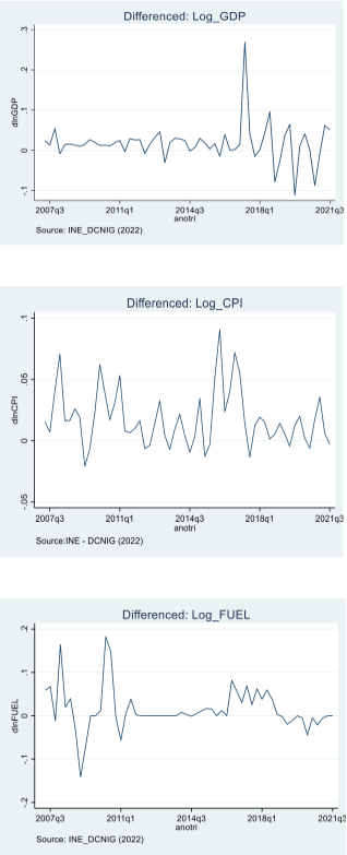
Figure 2. Average quarter prices of GDP, CPI and FUEL prices (Jan2016 -July2022).
Table 2. Descriptive statistics.

Variables

FUEL

CPI

GDP

N

59

59

59

Mean

44,90271

234,66570

133906,20000

Median

39,70849

241,39110

137675,90000

Skewness

0,48004

-0,35771

-0,23343

Kurtosis

1,90777

1,76801

1,58354

Min

25,67753

48,20374

83998,67000

Max

67,14500

401,80000

171608,60000

Std.dev

12,76602

122,84220

29207,79000

The Figure 2 indicates the variation of GDP, FUEL prices and CPI, where are clearly visible the effects of exogenous shocks since 2016, which culminated in the slowdown in the growth of the Gross Domestic Product and high levels of CPI. The main factors are:
“(i) the suspension of external support to the State Budget and the balance of payment by cooperation partners; (ii) the increase in external public debt service; (iii) the prolonged drought in the south-central region of the country and the floods in the north-central regions of the country; (iv) the political-military tension in the north-central region of the country, and (v) the drop in foreign direct investment (FDI)” .
Table 3 reports unit root test results of the Augmented Dicky-Fuller test. At levels, all variables are non-stationary as the p-values are greater than a 0.05 level of significance. Therefore, the null hypothesis of no stationarity can’t be rejected. This means that the series exhibits a unit root. At first difference, all variables are stationary as the p-values are less than 0.05 level of significance. The null hypothesis is rejected at first difference at 0.01 significance level. Therefore, all variables reached the same order of integration at I (1) or first difference. The proceeding step is a test for cointegrating vectors or long run relationship using the Johansen cointegration approach to test whether the variables are integrated in the long-run.
The fuel prices have been rising and volatile, impacting on global economic stability. International oil prices fluctuated around US$ 20 per barrel in the 1990s before rising. Oil prices experienced a sharp upward trend to reach an all-time high of close to US$ 133 per barrel in July 2008, later decreased to US$ 41 per barrel by the end in December 2008. After that decline oil prices swelled again (with minor plunges in between) and averaged around US$ 116 per barrel in April 2011. Yet in the last quarter of 2014, there has been a deep fall in the price of oil close to US$ 30 per barrel in January 2016. Since June 2019 and associated with the COVID-19 pandemic, there was a decrease in oil prices reaching a minimum of US$21 in June 2020, and then the prices returned to an upward trajectory up to US$117 in June 2022, (Figure 3).
Table 3. Unit root test.

Augmented Dickey-Fuller (ADF) - Unit Root Tests

Variables

Lags

Level: I(0)

First difference: I(1)

Order of integration result

t - Stat P-value

Conclusion at 5%

t - Stat P-value Conclusion at 5%

LnCPI

0

-1,593 0.7953

No Stationary

-7,5110 0,000 Stationary

I (1)

LnGDP

1

0,181 0,9957

No Stationary

-8,8780 0,000 Stationary

I (1)

LnFuel

0

-3,049 0.119

No Stationary

-4,4340 0,0019 Stationary

I (1)

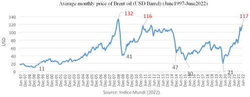
Figure 3. Average monthly price of Brent oil (USD/Barrel (June1997 -June2022).
However, Figure 4 show that the volatility of barrel prices in international market does not entirely been passed on the Mozambican customer because the government adopted fuel price control policy, which implies the maintenance of prices, at least for some times, and compensation to companies’ fuel distributors , 34]. The application of subsidies also occurs in Nigeria, which is a country producing and exporting oil. In Nigeria the retail prices are subsidized by the government and the subside is high or low depending on the international price of oil which is set by Organization of the Petroleum Exporting Countries (OPEC), and it was estimated that the government pays an amount of $2.5 billion U.S. dollars as subsidies, consequently resulting into price instability of oil products . This is because Nigeria is at the same time producer, exporter and importer of petroleum products, in such way that the macroeconomics variables such as exchange rate policy are be blamed for the level of inflation rate .
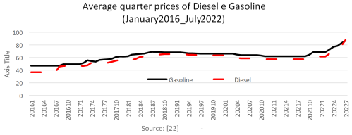
Figure 4. Average quarter prices of diesel e gasoline (MZN/Litre (Jan2016 -July2022).
4.2. Cointegration Results
Prior to conducting the Johansen cointegration test, a lag order selection process was used to select and determine the number of lags to be used in this test, including the vector error correction model (VECM). The optimal lag selection was based on five selection criteria, namely; LR, FPE, AIC, SCBIC and HQIC, where all criteria reached the same conclusion of two (1) lags for FUEL, three (3) for GDP and four (0) for CPI.
Table 5 reports results for the Trace test and Max-Eigenvalue statistics in the Johansen cointegration test. Both tests show one co-integrating equation (r≤1) at 0.05 level of significance. Thus, the null hypothesis of no co-integrating equation is rejected. This suggests that variables are co-integrated or that a long -run relationship exists within the series.
Table 4. Selection of lags.

Lag

Sample: 2008q1 thru 2021q3

Number of obs = 55

LL

LR

df

P

FPE

AIC

HQIC

SBIC

GDP

0

159,681

0,000164

-5,87709

-5,86289

-5,84026*

1

159,682

0,00032

1

0,986

0,00017

-5,84006

-5,81165

-5,76639

2

159,848

0,33304

1

0,564

0,000176

-5,80919

-5,76657

-5,69869

3

164,099

8,5024*

1

0,004

,000156*

-5,9296*

-5,87278*

-5,78227

4

164,755

1,3121

1

0,252

0,000158

-5,91687

-5,84584

-5,7327

ICP

0

24,1694

,024823*

-,858126*

-,843921*

-,821293*

1

24,1701

0,00145

1

0,97

0,025759

-0,82112

-0,79271

-0,74745

2

24,1947

0,04915

1

0,825

0,026709

-0,78499

-0,74237

-0,67449

3

24,1949

0,00046

1

0,983

0,027721

-0,74796

-0,69114

-0,60063

4

24,2152

0,04056

1

0,84

0,028753

-0,71167

-0,64065

-0,52751

FUEL

0

89,8605

0,002179

-3,29113

-3,27692

-3,25429

1

96,4294

13,138*

1

0

,001773*

-3,49739*

-3,46898*

-3,42372*

2

97,3715

1,8842

1

0,17

0,001777

-3,49524

-3,45263

-3,38474

3

97,6532

0,56339

1

0,453

0,001825

-3,46864

-3,41182

-3,32131

4

98,547

1,7876

1

0,181

0,001833

-3,4647

-3,39368

-3,28054

Table 5. Cointegration test.

Johansen tests for cointegration

Trend: Constant

Number of observations = 57

Sample: 2007q3 thru 2021q3

Number of lags =2

H0: No Cointegration

Maximum

Trace

Rank

Params

LL

Eigenvalue

Trace test - Critical value (5%)

Critical Value (5%)

0

12

315,53716

46,1952

29,68

1

17

332,2763

0,4442

12,7169

15,41 *

2

20

336,26006

0,13045

4,7494

3,76

3

21

338,63477

0,07995

Maximum

Params

LL

Eigenvalue

Maximum- Eigenvalue

Critical Value (5%)

Rank

0

12

315,53716

33,4783

20,97

1

17

332,2763

0,4442

7,9675

14,07*

2

20

336,26006

0,13045

4,7494

3,76

3

21

338,63477

0,07995

* Reject the null hypothesis, so there is at most one cointegration equation
4.3. Long-Term Relationships Between GDP, CPI and FUEL
In an attempt to assess the stability of the long-run relationship among the variables, the study adopts the Vector Error Correction Model (VECM). The purpose of VECM is to indicate the speed of adjustment from the short run equilibrium to the long-run equilibrium state.
The existence of a cointegrating relationship between the selected variables explain the long-run equilibrium.
𝐸𝐶𝑇𝑡−1 = [𝑦𝑡−1 𝑗𝑋𝑡−1 − 𝜉𝑚𝑅𝑡−1]. From table 6, the he cointegration equation and long-run model.
ECTt-1=[1. ln GDPt-1 + 0.3284 lnCPIt-1 - 0.4415 ln F uel - 11.66672]-value =                             0.0000                          0.000                                  (9)
In the long-run (Equation 9) with LNGDP as the dependent variable, illustrates that the CPI and FUEL prices have a symmetric and significant effects on GDP in the long run, in average, coeteris paribus. Specifically, this means that a one percentage changes in CPI and FUEL prices lead to an increase in GDP by 0.33% and decrease in 0.44%, respectively, coeteris paribus.
ECTt-1=[1.  CPIt-1+3.045GDPt-1 +1.344 ln F uel+35,52577]-value =                      0.0000                   0.000                             (10)
In the long-run (Equation 10) with LNCPI as the dependent variable, both the GDP and FUEL prices have a positive and significant impact on CPI on the long run, in average, coeteris paribus. Specifically, this means that a one percentage changes in GDP and FUEL prices lead to an increase in CPI by 3.045% and 1.344, respectively, coeteris paribus.
The results of this study, that show a negative impact of the rise in fuel prices on GDP, are similar to those obtained in India . However, this finding is not consistent with other authors , that showed crude oil prices as having a negative effect on GDP growth.
The reason behind the inverse relationship between the two variables is that, crude oil prices have an adverse effect on the manufacturing sector as it is a key input and therefore leading to a reduced production in industrial goods which impacts GDP growth in the long run expected the study found crude oil prices to have a positive effect on inflation in the long run .
Table 6. Long-run causality.

Long Run Equation

D (LNCPI)

D (LNFUEL)

D (LNGDP)

Coef

P-value

Coef

P-value

Coef

P-value

Constant

35,52577

-26,42498

-11,66672

CPI

1

-0,74383

0,00000

-0,32840

0,00000

FUEL

-1,34440

0,00000

1

0,44150

0,00000

GDP

-3,04505

0,00000

2,26499

0,00000

1

ECT

-0.04769

0.052

-0.02166

0.0216

-0.03538

0.010

Here, the Error Correction Mechanism (ECM) is estimated to ascertain how well the short-run dynamics in the model are adjusted on the long-run equilibrium path. The Table 5 illustrates that GDP, CPI and FUEL have joint long run equilibrium because have a negative Error Correction Term (ECT). A positive sign of error correction term indicates that the systems in the model are moving away from equilibrium .
4.4. Short-Term Relationships Between GDP, CPI and FUEL
The VECM output (Table 7) indicates that ECT constitutes one significant equation which explain short-run adjustment towards the long-run equilibrium and that is LNGDP. LNGDP has a negative coefficient (-0.03538) and p-value of 0.010, meaning that the variable is significant at 0.05 significance level. Also, the results in Table 7 suggests that previous quarter’s errors (or deviation from long-run equilibrium) are corrected for with the current quarter at a convergence speed of 3.5%, or in other words, the results suggests that 3.5% of the short-run errors will be corrected in the long-run equilibrium path.
The LNCPI has a negative coefficient (-0.04769) and p-value of 0.052, meaning that the variable is significant at 0.10 significance level, suggesting that previous quarter’s errors (or deviation from long-run equilibrium) are corrected for with the current quarter at a convergence speed of 4.8%, or in other words, the results suggests that 4.8% of the short-run errors will be corrected in the long-run equilibrium path.
The short-run results, in Table 6, indicate that increase in LNFUEL prices has a negative and not significant impact on GDP and positive but insignificant impact on CPI. These results are also consistent with most empirical literature that shows that increases in crude oil prices have a negative effect on GDP and positive effect on CPI in both long run and short run . Parallel, the LNCPI has a positive impact on GDP. Although both CPI and FUEL has no significant coefficients. On the other hand, previous changes in GDP has a positive, but not significant impact on GDP.
Table 7. Vector Error Correction Model.

Vector Correction Model

ERROR CORRECTION

D (LNCPI)

D (LNFUEL)

D (LNGDP)

Coef

P-value

Coef

P-value

Coef

P-value

CoinEq,1 (ECT)

-0,04769

0,0518***

-0,02166

0,0206**

-0,03538

0,01*

D(LNCPI-1)

-0,04871

0,754

0,03396

0,470

-0,05513

0,00*

D(LnFUEL-1)

-0,12061

0,775

0,41819

0,775

0,03257

0,185

D(LNGDP-1)

1,91465

0,336

-0,46852

0,436

0,16252

0,161

CONSTANT

0,00853

0,804

0,01539

0,138

0,01369

0,00*

* Significant at 1%; ** Significant at 5%; *** Significant at 10%
4.5. Short-term Relationships between GDP, CPI and FUEL
The existence of cointegration implies the existence of Granger causality at least in one direction (Granger, 1988). To confirm these short-run results, Granger causality tests were conducted and the results are listed in Table 8. Like findings in some Asia countries ; in Mozambique there is not a cointegrating long-run relationship between FUEL prices and CPI and GDP, which suggest that the impact of oil shocks on these variables is limited to the short-run.
When analyzing short-run relationship between fuel prices and CPI and GDP, oil prices shocks are found to Granger cause GDP and CPI, as all. Granger causality tests also indicate causality between CPI and GDP, and the results shows that the changes in GDP causes changes in other variables, CPI and FUEL respectively.
Table 8. Pairwise Granger Causality Results.

Pairwise Granger Causality Results

Null hypothesis

Chi-Square

p-value

Conclusion

GDP dos not Granger cause CPI

25,054

0,0000

Reject H0

GDP dos not Granger cause FUEL

0,70896

0,4000

Don’t Reject H0

GDP dos not Granger cause All

32,159

0,0000

Reject H0

CPI dos not Granger cause GDP

0,53597

0,4640

Don’t Reject H0

CPI dos not Granger cause FUEL

0,03792

0,8460

Don’t Reject H0

CPI dos not Granger cause All

0,55498

0,7580

Don’t Reject H0

FUEL dos not Granger cause GDP

0,24453

0,6210

Don’t Reject H0

FUEL dos not Granger cause CPI

0,66309

0,4150

Don’t Reject H0

FUEL dos not Granger cause All

0,55498

0,7110

Don’t Reject H0

4.6. Variance Decomposition (VDC) Analysis
The VDC provides a tool of analysis to determine the relative importance of real oil price shock in explaining the volatility of the three macroeconomic variables. The results showed that among the impact itself is the first source of variance, which is the most obvious in the first period, accounted for 100% for GDP, 68.66% for CPI and 99.94% for FUEL. With prolonged periods, the fluctuations gradually reduced the impact on its own, and in the long-term (8 quarters) it seems there is 59.22% for GDP, 56.29% for CPI and 98.016% for GDP. CPI is the variable with the highest explanatory power over the variation in FUEL prices, Increases by 1.4% in the first quarter to 19.03% in 8th quarter. Shocks in CPI explain about 29.68% of GDP and 0.93% in FUEL in 8TH quarter. Also, the results of the VDC suggest that an FUEL price shock is not a major source of volatility of CPI and GDP in Mozambique. As shown in table 9, FUEL price shock is a minimal source of disturbance to GDP and CPI reaching in 8th quarter, only 11.10% and 19.03%, respectively.
Table 9. Variance decomposition (VDC) analysis.

Impulse

lnGDP

lnGDP

lnGDP

lnCPI

lnCPI

lnCPI

lnFUEL

lnFUEL

lnFUEL

Response

lnGDP

lnCPI

lnFUEL

lnGDP

lnCPI

lnFUEL

lnGDP

lnCPI

lnFUEL

1

2

3

4

5

6

7

8

9

Step

fevd

fevd

fevd

fevd

fevd

fevd

Fevd

fevd

fevd

0

0,0000

0,0000

0,0000

0,0000

0,0000

0,0000

0,0000

0,0000

0,0000

1

1,0000

0,2995

0,0006

0,0000

0,6866

0,0000

0,0000

0,0139

0,9994

2

0,6655

0,2876

0,0009

0,3248

0,6606

0,0047

0,0097

0,0517

0,9944

3

0,6175

0,2519

0,0078

0,3010

0,5762

0,0104

0,0815

0,1719

0,9818

4

0,6001

0,2466

0,0091

0,2984

0,5641

0,0105

0,1015

0,1893

0,9804

5

0,5931

0,2467

0,0092

0,2969

0,5634

0,0105

0,1100

0,1899

0,9803

6

0,5929

0,2469

0,0092

0,2971

0,5633

0,0105

0,1099

0,1899

0,9802

7

0,5922

0,2468

0,0093

0,2968

0,5630

0,0106

0,1109

0,1902

0,9802

8

0,5922

0,2468

0,0093

0,2968

0,5629

0,0106

0,1110

0,1903

0,9801

4.7. Impulse and Response Analyse
Figure 5 shows the series impulse responses are used to trace out the dynamic effects of an unanticipated shock on GDP, CPI and FUEL prices. The horizontal axis represents the number of quarters (in this case eight quarters) and the vertical axis represents the magnitude of the reaction of the variables considered in the face of an unexpected shock, increase or decrease of the variable of interest. There are nine situations divided into three figures. So, in the first line we have impulse in the CPI and responses in the CPI itself, then in the FUEL and finally in the GDP. In the second line, we have impulse in FUEL and responses in CPI, in FUEL itself and in GDP. In the last line we have impulse in GDP and responses in CPI, FUEL and in GDP itself.
The analysis of impulse responses shows that CPI are relatively more sensitive to unexpected shocks to each of the variables, reaching equilibrium and stability, at most, up to the fourth quarter. For example, a shock, an increase in fuel prices, leads to increases in CPI, but from the third quarter onwards there is stability. On the other hand, the GDP have a stability due the schoks in CPI and FUEL prices.
4.8. Diagnostics Tests
The model passed diagnostic tests of no heteroscedasticity, no serial correlation, and normality with results showing that the residual is not normal distribution, has serial correlation and are not homoscedasticity, Table 10.
Table 10. Diagnostics tests.

Test Null Hypothesis Chi-square Probability Decision

LM Test

No serial correlation

31.30

0.000

With p-value less than 5%, reject H0. Therefore, the results show that there is serial correlation in the model

White Test

No heteroscedasticity

21.56

0.000

With p-value less than 5%, reject H0. Therefore, the results show that there is a heteroscedasticity in the model

Jarque-Bera

Residual are normal distributed

78.7453

0.000

With p-value less than 5%, reject H0. Therefore, the results show that the data is not normally distributed

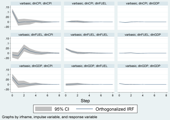
Figure 5. Impulse and Response.
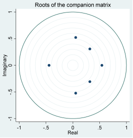
Figure 6. Root test estimates.
Figure 6 reports the inverse root graph. The study plotted the AR inverse root graph to establish the stability and reliability of the IRF and the robustness of the VECM model. The outcome of the inverse roots graph confirms the stability of the model as all AR roots lie within the unit circle.
5. Conclusion
The main objective of this study was to determine the impact of changes in the FUEL price on CPI and GDP in Mozambique, and was achieved by means of a comprehensive literature review and also through the use of a quantitative analysis of time series data for Mozambique. The most important results are that in Mozambique there are a cointegrating long-run relationship between FUEL prices and CPI and GDP, which suggest that the impact of FUEL prices shocks to CPI and GDP in short-run and long-run path. Also in the long run, the GDP have joint long run price transmission with CPI and FUEL.
In the long-run with LNCPI as the dependent variable, both the GDP and FUEL prices have a positive and significant impact on CPI on the long run, in average, coeteris paribus. Specifically, this means that a one percentage changes in GDP and FUEL prices lead to an increase in CPI by 3.045% and 1.344, respectively, coeteris paribus. The LNGDP has a negative coefficient (-0.03538) and p-value of 0.010, meaning that the variable is significant at 0.05 significance level. Also, the results in Table 5 suggests that previous quarter’s errors (or deviation from long-run equilibrium) are corrected for with the current quarter at a convergence speed of 3.5%, or in other words, the results suggests that 3.5% of the short-run errors will be corrected in the long-run equilibrium path. In the other hand, the LNCPI has a negative coefficient (-0.04769) and p-value of 0.052, meaning that the variable is significant at 0.10 significance level, suggesting that previous quarter’s errors (or deviation from long-run equilibrium) are corrected for with the current quarter at a convergence speed of 4.8%, or in other words, the results suggests that 4.8% of the short-run errors will be corrected in the long-run equilibrium path.
The short-run results, indicate that increase in LNFUEL prices has a negative and not significant impact on GDP and positive but insignificant impact on CPI. When analyzing short-run relationship between fuel prices and CPI and GDP, oil prices shocks are found to Granger cause GDP and CPI, as all. Granger causality tests also indicate causality between CPI and GDP, and the results shows that the changes in GDP causes changes in other variables, CPI and FUEL respectively.
The VDC provides a tool of analysis to determine the relative importance of real oil price shock in explaining the volatility of the three macroeconomic variables. The results showed that among the impact itself is the first source of variance, which is the most obvious in the first period, accounted for 100% for GDP, 68.66% for CPI and 99.94% for FUEL. With prolonged periods, the fluctuations gradually reduced the impact on its own, and in the long-term (8 quarters) it seems there is 59.22% for GDP, 56.29% for CPI and 98.016% for GDP. CPI is the variable with the highest explanatory power over the variation in FUEL prices, Increases by 1.4% in the first quarter to 19.03% in 8th quarter. Shocks in CPI explain about 29.68% of GDP and 0.93% in FUEL in 8TH quarter. Also, the results of the VDC suggest that an FUEL price shock is not a major source of volatility of CPI and GDP in Mozambique. As shown in table 8, FUEL price shock is a minimal source of disturbance to GDP and CPI reaching in 8th quarter, only 11.10% and 19.03%, respectively.
The analysis of impulse responses shows that CPI are relatively more sensitive to unexpected shocks to each of the variables, reaching equilibrium and stability, at most, up to the fourth quarter. For example, a shock, an increase in fuel prices, leads to increases in CPI, but from the third quarter onwards there is stability. On the other hand, the GDP have a stability due the schoks in CPI and FUEL prices.
Abbreviations

CPI

Consumer Price Index

ECT

Error Correction Term

EU

European Union

ECM

Error Correction Mechanism

GDP

Gross Domestic Product

IMF

International Monetary Fund

IWGPS

Inter-secretariat Working Group on Price Statistics

ISWGNA

Inter-Secretariat Working Group on National Accounts

OECD

Organization for Economic Co-operation and Development

SNA

System of National Accounts

UN

United Nations

UNSD

The United Nations Statistics Division

VAR

Vector Autoregressive

VDC

Decomposition of Variance

VECM

Vector Error Correction Mechanism

WB

World Bank

Author Contributions
Sandre Macia: Conceptualization, Data curation, Formal Analysis, Investigation, Methodology, Resources, Software, Supervision, Validation, Visualization, Writing – original draft, Writing – review & editing
Júlio Macuacua: Validation, Writing – review & editing
Alfeu Vilanculos: Formal Analysis, Investigation, Supervision Validation
Filipe Mahaluça: Formal Analysis, Investigation, Methodology, Validation, Visualization
Conflicts of Interest
The authors declare no conflicts of interest.
References
[1] Akinleye, S. O., & Ekpo, S. (2013). Oil price shocks and macroeconomic performance in Nigeria. Economía Mexicana Nueva Época, volumen Cierre de época, número II de 2013, pp 565-624.
[2] Adeleye, N., Ogundipe, A. A., Ogundipe, O., Ogunrinola, I., & Adediran, O. (2019). Internal and external drivers of inflation in Nigeria. Banks Bank Syst, 14(4), 206-218. Pdf (semanticscholar.org).
[3] Arndt, C., Benfica, R., Maximiano, N., Nucifora, A. M., & Thurlow, J. T. (2008). Higher fuel and food prices: impacts and responses for Mozambique. Agricultural Economics, 39, 497-511.
[4] Arndt C, Matsinhe L, Mulder P, Paulo E, e Van Dunem J. (2005) “O impacto do aumento do preço do petróleo na Economia Moçambicana”. Ministerio da Planificacao e Desenolvimento, DNEAP Discussion paper, p. 19. 28.
[5] Arinze, P. E. (2011). The impact of oil price on the Nigerian economy. Journal of Research in National Development, 9(1), 211-215.
[6] Banco de Mocambique (2016). Relatorio Anual 2016. Maputo. Mocambique. Disponivel em:
[7] Bellemare, M. F. (2015). Rising food prices, food price volatility, and social unrest. American Journal of agricultural economics, 97(1), 1-21.
[8] Bhattacharya, K., & Bhattacharya, I. (2001). Impact of increase in oil prices on inflation and output in India. Economic and Political Weekly, 36(51), 4735–4741.
[9] Bobai, F. D. (2012). An analysis of the relationship between petroleum prices and inflation in Nigeria. International Journal of Business and Commerce, 1(12), 01–07.
[10] Brito, L. D. (2017). Agora eles têm medo de nós! Uma colectânea de textos sobre as revoltas populares em Moçambique (2008–2012). Maputo: IESE.
[11] Brinkman, C. S. Hendrix, Food insecurity and conflict: Applying the WDR framework, World Development Report 2011 (August 2, 2010).
[12] Brown, S. P., & Yücel, M. K. (2002). Energy prices and aggregate economic activity: an interpretative survey. The Quarterly Review of Economics and Finance, 42(2), 193-208.
[13] Chang, Y., & Wong, J. F. (2003). Oil price fluctuations and Singapore economy. Energy policy, 31(11), 1151-1165.
[14] Chamalwa, H. A., & Bakari, H. R. (2016). A Vector Autoregressive (VAR) Cointegration and Vector Error Correction Model (VECM) approach for financial deepening indicators and economic growth in Nigeria. American Journal of Mathematical Analysis, 4(1), 1-6.
[15] Commission of the European Communities, International Monetary Fund, Organisation for Economic Cooperation and Development, United Nations and World Bank, System of National Accounts 2008. Brussels/Luxembourg, Washington, D. C., Paris, New York, 2008. United Nations Publication, Sales No. E. 94.XVII. 4.
[16] Cunado, J., & De Gracia, F. P. (2005). Oil prices, economic activity and inflation: evidence for some Asian countries. The Quarterly Review of Economics and Finance, 45(1), 65-83.
[17] Du, L., Yanan, H., Chu, W & Wei, C. (2010). The relationship between oil price shocks and China’s macro-economy: An empirical analysis. Energy policy, 38(8), 4142-4151.
[18] Gbenga, O., & Omo-Ojugo, S. O. (2022). The Effect of Petroleum Product Prices Adjustment on Inflation Rate in Nigeria (1980-2021). Academic Journal of Digital Economics and Stability, 15, 164175.
[19] Gujarati DN (2003). Basic Econometrics. 4th Edition, McGraw-Hill, New York.
[20] Hamilton, J. D. (1983). Oil and the Macroeconomy since World War II, Journal of Political Economy, 91(3), 228-248.
[21] Inter-Secretariat Working Group on National Accounts (United Nations, European Commission, International Monetary Fund, Organisation for Economic Cooperation and Development and World Bank) – ISWGNA (2009), System of National Accounts 2008, Series F, No. 2, Rev. 5, United Nations, New York.
[22] Inter-secretariat Working Group on Price Statistics (International Labour Organization, International Monetary Fund, Organisation for Economic Co-operation and Development, European Union, United Nations and The World Bank) – IWGPS, (2020). Consumer price index manual: concepts and methods. International Monetary Fund, Publication, Washington, U.S.A.
[23] INE - Instituto Nacional de Estatística (2022). Contas Nacionais. Maputo- Moçambique.
[24] Jiménez-Rodríguez, R., & Sánchez, M. (2005). Oil price shocks and real GDP growth: empirical evidence for some OECD countries. Applied economics, 37(2), 201-228.
[25] Johansen, S., & Juselius, K. (1990). Maximum likelihood estimation and inference on cointegration— with appucations to the demand for money. Oxford Bulletin of Economics and statistics, 52(2), 169210.
[26] Kinyanjui, A. K. (2018). Effects of crude oil prices on gross domestic product growth and selected macroeconomic variables in kenya (doctoral dissertation, kenyatta university).
[27] Korhonen, I., & Ledyaeva, S. (2010). Trade linkages and macroeconomic effects of the price of oil. Energy Economics, 32(4), 848-856.
[28] Lepenies, P. (2016). The power of a single number: a political history of GDP. Columbia University Press.
[29] Le Blanc, M. & Chinn, M. (2004). Do high oil price presage inflation? The evidence from G-5 countries. Santa Cruz Center for International Economics (Working Paper, WP1021).
[30] Lagi, M., Bertrand, K. Z., & Bar-Yam, Y. (2011). The food crises and political instability in North Africa and the Middle East. arXiv preprint arXiv: 1108.2455.
[31] Lescaroux, F., & Mignon, V. (2008). On the influence of oil prices on economic activity and other macroeconomic and financial variables. OPEC Energy Review, 32(4), 343-380.
[32] Malik, A. (2016). The impact of oil price changes on inflation in Pakistan. International journal of energy economics and policy, 6(4), 727-737.
[33] Masiya, M. (2010). The Lisman and Sandee Method of Interpolation in Stata. Available at SSRN 2504523.
[34] Meyer, D. F. (2018). The impact of changes in fuel prices on inflation and economic growth in South Africa. In Proceedings of the 11th International RAIS Conference on Social Sciences (pp. 65-73). Scientia Moralitas Research Institute. http://rais.education/wp-content/uploads/2018/11/010DM.pdf
[35] Nhamire, B., Mapisse, I., & Fael, B. (2019). Corrupção e más práticas no sectores dos combustíveis e de energia eléctrica: seus efeitos para o orçamento das famílias moçambicanos. CIP, Centro de Integridade Pública.
[36] Ocheni, S. I. (2015). Impact of fuel price increaseon the Nigerian economy. Mediterranean Journal of Social Sciences, 6(1 S1), 560-560. Impact of Fuel Price Increaseon the Nigerian Economy | Mediterranean Journal of Social Sciences (richtmann.org).
[37] Peker, O., & Mercan, M. (2011). The inflationary effect of price increases in oil products in Turkey. Ega Academic Review, 11(4), 553–562.
[38] Przekota, G.; Szczepa ´nska-Przekota, A. Pro-Inflationary Impact of the Oil Market—A Study for Poland. Energies 2022, 15, 3045.
[39] Peersman, G., & Van Robays, I. (2012). Cross-country differences in the effects of oil shocks. Energy Economics, 34(5), 1532-1547.
[40] Sarmah, A., & Bal, D. P. (2021). Does Crude Oil Price Affect the Inflation Rate and Economic Growth in India? A New Insight Based on Structural VAR Framework. The Indian Economic Journal, 69(1), 123-139.
[41] Sek, S. K., Teo, X. Q., & Wong, Y. N. (2015). A comparative study on the effects of oil price changes on inflation. “4th World Conference on Business, Economics and Management, WCBEM”.
[42] Tang, W., Wu, L., & Zhang, Z. (2010). Oil price shocks and their short-and long-term effects on the Chinese economy. Energy Economics, 32, S3-S14.
Cite This Article
  • APA Style

    Macia, S., Macuacua, J., Vilanculos, A., Mahaluça, F. (2024). Impact of Changes in Fuel Prices on Inflation and Economic Growth in Mozambique. International Journal of Economics, Finance and Management Sciences, 12(3), 142-160. https://doi.org/10.11648/j.ijefm.20241203.12

    Copy | Download

    ACS Style

    Macia, S.; Macuacua, J.; Vilanculos, A.; Mahaluça, F. Impact of Changes in Fuel Prices on Inflation and Economic Growth in Mozambique. Int. J. Econ. Finance Manag. Sci. 2024, 12(3), 142-160. doi: 10.11648/j.ijefm.20241203.12

    Copy | Download

    AMA Style

    Macia S, Macuacua J, Vilanculos A, Mahaluça F. Impact of Changes in Fuel Prices on Inflation and Economic Growth in Mozambique. Int J Econ Finance Manag Sci. 2024;12(3):142-160. doi: 10.11648/j.ijefm.20241203.12

    Copy | Download

  • @article{10.11648/j.ijefm.20241203.12,
      author = {Sandre Macia and Júlio Macuacua and Alfeu Vilanculos and Filipe Mahaluça},
      title = {Impact of Changes in Fuel Prices on Inflation and Economic Growth in Mozambique
    },
      journal = {International Journal of Economics, Finance and Management Sciences},
      volume = {12},
      number = {3},
      pages = {142-160},
      doi = {10.11648/j.ijefm.20241203.12},
      url = {https://doi.org/10.11648/j.ijefm.20241203.12},
      eprint = {https://article.sciencepublishinggroup.com/pdf/10.11648.j.ijefm.20241203.12},
      abstract = {The fuel oil is a basic input to production, so an increase in oil price leads to a rise in production costs that induces firms to lower output. In parallel, oil prices change also effects, indirectly, the consumption, through its positive relation with disposable income. However, despite the relevance of the variation in fuel prices in economy, there are no recent study conducted to analyse the impact of changes in fuel prices on GDP and CPI in Mozambique. This study aims to contribute to filling the information gap by providing the quantification of the impact of fuel prices on GDP and CPI. So, the study aim to determine the impact of changes in FUEL prices on Inflation (Consumer Price Index – CPI) and Economic Growth (Gross Domestic Product – GDP), using quarter data from 2007 to 2020. Descriptive statistics, Unit Root Test, Johansen Cointegration Test and Error Correction Model, Granger Causality Econometric Models, Impulse and Response Function and Variance Decomposition Analysis are used. The results indicate that in Mozambique there are a cointegrating long-run relationship between FUEL prices and CPI and GDP, which suggest that the impact of FUEL prices shocks to CPI and GDP in short-run and long-run path. Also, the results show that changes in GDP and FUEL prices lead to an increase in CPI by 3.0% and 1.3%, respectively, coeteris paribus. The previous quarter’s errors (or deviation from long-run equilibrium) are corrected for with the current quarter at a convergence speed of 3.5% to GDP, and 4.8% to CPI. Granger causality tests also indicate causality between CPI and GDP, and the changes in GDP causes changes in other variables.
    },
     year = {2024}
    }
    

    Copy | Download

  • TY  - JOUR
    T1  - Impact of Changes in Fuel Prices on Inflation and Economic Growth in Mozambique
    
    AU  - Sandre Macia
    AU  - Júlio Macuacua
    AU  - Alfeu Vilanculos
    AU  - Filipe Mahaluça
    Y1  - 2024/05/30
    PY  - 2024
    N1  - https://doi.org/10.11648/j.ijefm.20241203.12
    DO  - 10.11648/j.ijefm.20241203.12
    T2  - International Journal of Economics, Finance and Management Sciences
    JF  - International Journal of Economics, Finance and Management Sciences
    JO  - International Journal of Economics, Finance and Management Sciences
    SP  - 142
    EP  - 160
    PB  - Science Publishing Group
    SN  - 2326-9561
    UR  - https://doi.org/10.11648/j.ijefm.20241203.12
    AB  - The fuel oil is a basic input to production, so an increase in oil price leads to a rise in production costs that induces firms to lower output. In parallel, oil prices change also effects, indirectly, the consumption, through its positive relation with disposable income. However, despite the relevance of the variation in fuel prices in economy, there are no recent study conducted to analyse the impact of changes in fuel prices on GDP and CPI in Mozambique. This study aims to contribute to filling the information gap by providing the quantification of the impact of fuel prices on GDP and CPI. So, the study aim to determine the impact of changes in FUEL prices on Inflation (Consumer Price Index – CPI) and Economic Growth (Gross Domestic Product – GDP), using quarter data from 2007 to 2020. Descriptive statistics, Unit Root Test, Johansen Cointegration Test and Error Correction Model, Granger Causality Econometric Models, Impulse and Response Function and Variance Decomposition Analysis are used. The results indicate that in Mozambique there are a cointegrating long-run relationship between FUEL prices and CPI and GDP, which suggest that the impact of FUEL prices shocks to CPI and GDP in short-run and long-run path. Also, the results show that changes in GDP and FUEL prices lead to an increase in CPI by 3.0% and 1.3%, respectively, coeteris paribus. The previous quarter’s errors (or deviation from long-run equilibrium) are corrected for with the current quarter at a convergence speed of 3.5% to GDP, and 4.8% to CPI. Granger causality tests also indicate causality between CPI and GDP, and the changes in GDP causes changes in other variables.
    
    VL  - 12
    IS  - 3
    ER  - 

    Copy | Download

Author Information
  • Abstract
  • Keywords
  • Document Sections

    1. 1. Introduction
    2. 2. Literature Review
    3. 3. Methodology
    4. 4. Results
    5. 5. Conclusion
    Show Full Outline
  • Abbreviations
  • Author Contributions
  • Conflicts of Interest
  • References
  • Cite This Article
  • Author Information