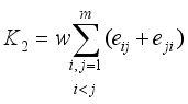
Practical problems in mixture experiments are usually associated with the investigation of mixture of m ingredients, which are assumed to influence the response through the proportions in which they are blended together. Mixture experiments are modeled using Scheffe’ models or Kronecker models whichever that is applicable. In such problems, the response of mixture experiments may also be affected by the conditions under which the mixture in conducted. This creates a shift in the blending characteristics of the mixture ingredients hence affecting the end product hence the need for inclusion of these conditions during modeling of mixture experiments. The objective of this study is to construct D-optimal designs for mixture experiments in the presence of process variables. In order to achieve this, first, a combined model of the second-degree Kronecker model for mixture experiments and the second-degree polynomial in the process variables in developed. The D-optimal designs are constructed using a Monte Carlo algorithmic approach in the AlgDesign of the R-packages. The designs constructed in this study were augmented with two replications of a level of the process variable. The D-optimal designs are evaluated using their D-optimal values and their relative D-efficiencies. The results of this study illustrate the existence of two alternate designs; one replicating at (-1, -1) and (-1, 1) in Table 2 and the other replicating at (0, 0) in Table 1. In conclusion the results of this study indicate that a design replicating at different levels of the process variable performs better than the one replicating at the overall centroid.
| Published in | American Journal of Theoretical and Applied Statistics (Volume 14, Issue 5) |
| DOI | 10.11648/j.ajtas.20251405.13 |
| Page(s) | 236-249 |
| Creative Commons |
This is an Open Access article, distributed under the terms of the Creative Commons Attribution 4.0 International License (http://creativecommons.org/licenses/by/4.0/), which permits unrestricted use, distribution and reproduction in any medium or format, provided the original work is properly cited. |
| Copyright |
Copyright © The Author(s), 2025. Published by Science Publishing Group |
Mixture Experiment, Mixture Ingredients, Process Variables, Kronecker Product, Moment Matrix, D-Optimal
 be the unity vector, whence,
  is the sum of the ingredients of t. Therefore, the experimental conditions are points in the probability simplex, which constitute the independent and controlled variables with the experimental domain being the simplex,
  . Under experimental conditions
  , the experimental response Yt is taken to be a scalar random variable. Replications under identical experimental conditions or response from distinct experimental conditions are assumed to be of equal (unknown) variance,
  , and uncorrelated. An experimental design is a probability measure on the experimental domain with finite support points of. If assigns weights w1, w2,… to its points of support in , then the experimenter is directed to draw proportions w1, w2,… of all observations under the respective experimental conditions.
  on the matrix of all cross products:
  ,
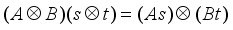
,  . The benefits enjoyed are; that distinct terms are repeated appropriately according to the number of times they can arise, that transformational rules with a conformable matrix R become simple,
 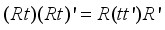 and that the approach extends to third degree polynomial regression.
  matrix A and a
  matrix B, their Kronecker product
  is defined to be the
  block matrix
 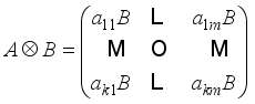 .
.  and another vector
  then is simply a special case
 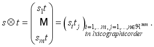 .
.  .
.  for Moore-Penrose inversion,
  and if possible for regular inversion
  .
.  is also an orthogonal matrix.
  assembles the cross products
  in an
in an  array, the Kronecker square
  arranges the same numbers as a long
  vector. The transformation with a conformable matrix R simply amounts to
 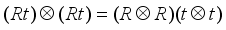 . This greatly facilitates the calculations we apply to response surface models.
  is provided by Kiefer’s
  , with
  . These are defined by;
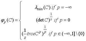
 matrices. Here
  stands for the smallest eigenvalue of C. By definition,
  is a function of the eigenvalues of C for all
  Pukelsheim
  includes the often used T-, D-, A-, and E-criteria, corresponding to parameter values 1, 0, -1, and
  respectively.
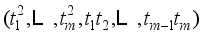
  , the m2x1 vector consisting of the squares and cross products of the components of t in the lexicographic order of the subscripts. This is referred to as Kronecker-model with a Kronecker-polynomial as the regression function
 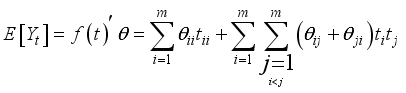 (1)
(1)  designs in that model. Draper, Heiligers and Pukelsheim
  weighted centroid designs for
  by adopting the general equivalence theorem as given in Pukelsheim
  .
.  , the second-degree Kronecker model for this experiment is given by
 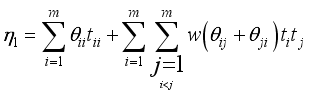 (2)
(2)  , and therefore has
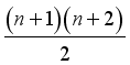
  terms in the mixture ingredients.
  process variables
  .
. 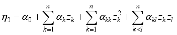 (3)
(3)  terms in the process variables. Crossing the terms of model in equation (2) with model in equation (3) results in a combined Kronecker mixture process variable model as shown below
 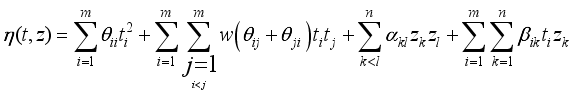 (4)
(4)  terms namely, the pure quadratic terms of the mixture ingredients, two-mixture ingredient interaction terms of the mixture ingredients, two-factor interaction of the process variables and the interaction between ingredients and the one-way interaction between the ingredients and the process variables.
  mixture ingredients and
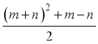
  process variables. First a data frame consisting of the name of each variable, the limits, number of levels and the center points are specified. Using Monte Carlo algorithm, a D-Optimal split-plot design for the model equation (4) consisting of
  design points arranged into
  whole plots each consisting of
  subplots is constructed. The first design involves replicating the overall centroid of the mixture ingredient at the center of the process variables. The process involves combining algorithmic design construction and inclusion of center points. For first design, the algorithm resulted in the design in Table 1 as shown below.
 Runs |
|
|
|
|
|
|---|---|---|---|---|---|
1 | 0 | 1 | 0 | -1 | -1 |
2 | 1 | 0 | 0 | -1 | -1 |
3 | 0 | 0 | 1 | -1 | -1 |
4 | 0.5 | 0 | 0.5 | -1 | -1 |
5 | 0 | 0 | 1 | -1 | 1 |
6 | 0 | 1 | 0 | -1 | 1 |
7 | 0.5 | 0.5 | 0 | -1 | 1 |
8 | 1 | 0 | 0 | -1 | 1 |
9 | 0 | 0 | 1 | 1 | -1 |
10 | 1 | 0 | 0 | 1 | -1 |
11 | 0.5 | 0.5 | 0 | 1 | -1 |
12 | 0 | 0.5 | 0.5 | 1 | -1 |
13 | 0 | 0 | 1 | 1 | 1 |
14 | 1 | 0 | 0 | 1 | 1 |
15 | 0.5 | 0 | 0.5 | 1 | 1 |
16 | 0 | 1 | 0 | 1 | 1 |
17 | 1/3 | 1/3 | 1/3 | 0 | 0 |
18 | 1/3 | 1/3 | 1/3 | 0 | 0 |
19 | 1/3 | 1/3 | 1/3 | 0 | 0 |
20 | 1/3 | 1/3 | 1/3 | 0 | 0 |
21 | 1/3 | 1/3 | 1/3 | 0 | 0 |
22 | 1/3 | 1/3 | 1/3 | 0 | 0 |
23 | 1/3 | 1/3 | 1/3 | 0 | 0 |
24 | 1/3 | 1/3 | 1/3 | 0 | 0 |
25 | 1/3 | 1/3 | 1/3 | 0 | 0 |
26 | 1/3 | 1/3 | 1/3 | 0 | 0 |
27 | 1/3 | 1/3 | 1/3 | 0 | 0 |
28 | 1/3 | 1/3 | 1/3 | 0 | 0 |
Runs |
|
|
|
|
|
|---|---|---|---|---|---|
1 | 0 | 1 | 0 | -1 | -1 |
2 | 1 | 0 | 0 | -1 | -1 |
3 | 0 | 0 | 1 | -1 | -1 |
4 | 0.5 | 0 | 0.5 | -1 | -1 |
5 | 0 | 1 | 0 | -1 | -1 |
6 | 1 | 0 | 0 | -1 | -1 |
7 | 0 | 0 | 1 | -1 | -1 |
8 | 0.5 | 0 | 0.5 | -1 | -1 |
9 | 0 | 0 | 1 | -1 | 1 |
10 | 0 | 1 | 0 | -1 | 1 |
11 | 0.5 | 0.5 | 0 | -1 | 1 |
12 | 1 | 0 | 0 | -1 | 1 |
13 | 0 | 0 | 1 | -1 | 1 |
14 | 0 | 1 | 0 | -1 | 1 |
15 | 0.5 | 0.5 | 0 | -1 | 1 |
16 | 1 | 0 | 0 | -1 | 1 |
17 | 0 | 0 | 1 | 1 | -1 |
18 | 1 | 0 | 0 | 1 | -1 |
19 | 0.5 | 0.5 | 0 | 1 | -1 |
20 | 0 | 0.5 | 0.5 | 1 | -1 |
21 | 0 | 0 | 1 | 1 | 1 |
22 | 1 | 0 | 0 | 1 | 1 |
23 | 0.5 | 0 | 0.5 | 1 | 1 |
24 | 0 | 1 | 0 | 1 | 1 |
25 | 1/3 | 1/3 | 1/3 | 0 | 0 |
26 | 1/3 | 1/3 | 1/3 | 0 | 0 |
27 | 1/3 | 1/3 | 1/3 | 0 | 0 |
28 | 1/3 | 1/3 | 1/3 | 0 | 0 |
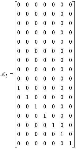
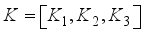
 mixture ingredients, let
  and
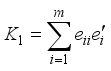
and  process variables, that is, a combined MPV model of three mixture ingredients and two process variables. In order to obtain the moment matrix and the information matrix for the design in Table 1, the coefficient matrix K for the parameter subsystem of interest as follows;
 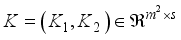 (5)
(5)  ,
,  ,
,  is the number of estimable parameters, and
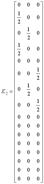
  is a prior weight defined by the experimenter. However, K may be extended by use of the matrices
  where necessary. Let
  ,
,  and
and  be defined as follows;
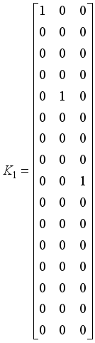
 we find that
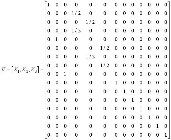
 is obtained as follows
 is given by
  , where,
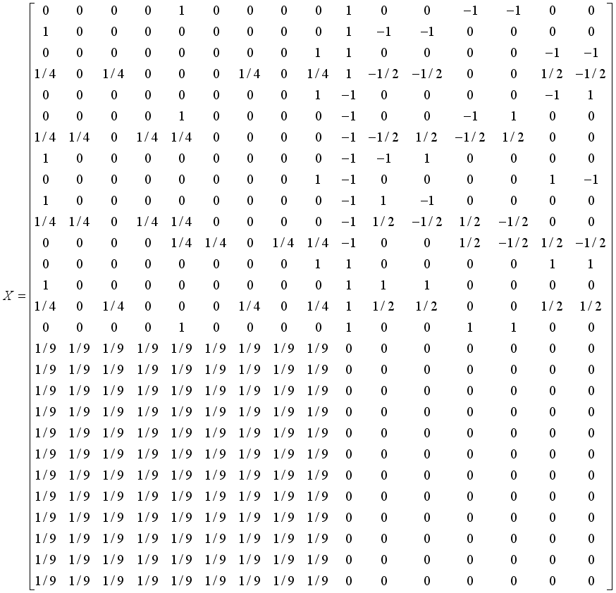
  . For the design given in Table 1, the
  matrix is given by
 the information matrix now becomes
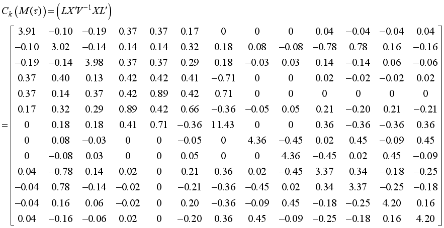

 the information matrix now becomes
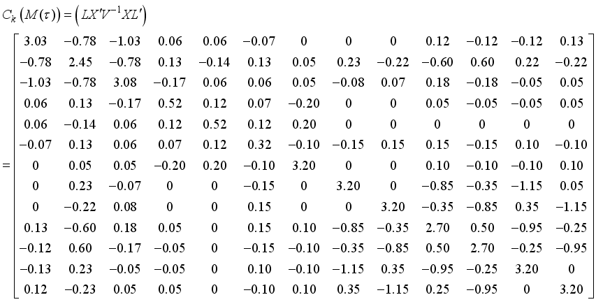

 the information matrix now becomes
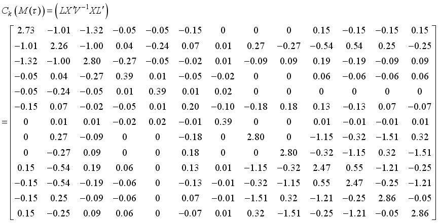

 mixture ingredients, let
  and
and  process variables, that is, a combined MPV model of three mixture ingredients and two process variables. In order to obtain the moment matrix and the information matrix for the design in Table 2, the coefficient matrix K for the parameter subsystem of interest as obtained before, then the design matrix based on the second-degree Kronecker model for mixture experiments for three mixture ingredients and two process variables for the design in Table 2 is given by
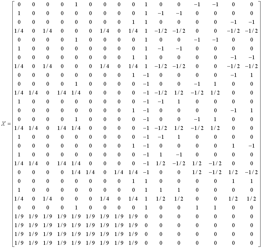
 is given by
 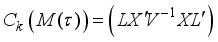 , where,
 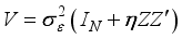 .
.  matrix is given by
 the information matrix now becomes
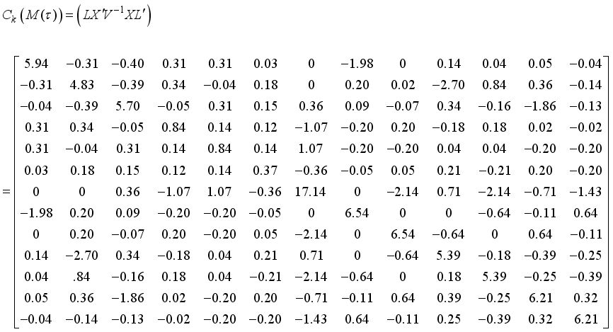

 the information matrix now becomes
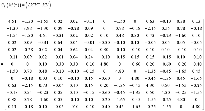

 the information matrix now becomes
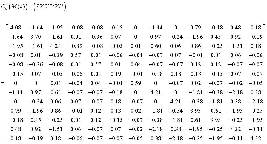

 .
. 
 and
and  are the model design matrices of the two competing designs.
  be the design matrix of the design in Table 1 and
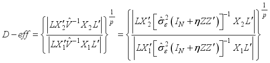
  be the design matrix of the design in Table 2, making use of this computation approach, the D-efficiencies for variance ratio
  is computed as follows:
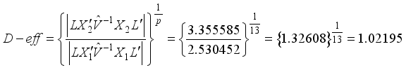
 is computed as follows:
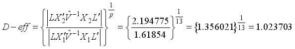
 is computed as follows:
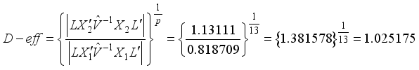
A | Average |
C | Information matrix |
D | Determinant |
E | Eigenvalue |
MPV | Mixture process variable |
PD | Positive Definite |
T | Trace |
| [1] | Chan, L. Y. (2000). “Optimal Designs of Experiments with Mixtures: a survey.” Communications in statistics-theory and methods, Vol. 29(9 & 10), 2281-2312. |
| [2] | Cornell, J. A. (1971). “Process Variables in the Mixture Problems Categorized.” J. Amer. Statist. Assoc Vol. 66: 42-88. |
| [3] | Cornell, J. A. (2002). “Experiments with mixtures: Designs, Models and the Analysis of Mixture Data”. Third Edition, John Wiley and Sons, New York. |
| [4] | Czitrom, V. (1988) “Mixture experiments with Process Variables: D-Optimal Orthogonal Experimental Designs.” Communications in statistics-theory and methods, Vol. 17: 105-121, |
| [5] | Czitrom, V. (1989) “Experimental Design for Four Mixture Components with Process Variables” Communications in statistics-theory and methods, Vol. 18: 4561-4581. |
| [6] | Draper, N. R. and Pukelsheim, F., (1998). Kiefer ordering of simplex designs for first-and second degree mixture models. In: Journal of statistical planning and inference, vol. 79: 325-348. |
| [7] | Draper, N. R., Heilingers, B., Pukelsheim, F. (2000). Kiefer ordering of simplex designs for mixture models with four or more ingredients. In: Annals of statistics, vol. 28: 578-590. |
| [8] | Galil, Z., Kiefer J. (1977). “Comparison of Simplex Designs for Quadratic Mixture” Technometrics, Vol 19, 445-453. |
| [9] | Goldfarb, H. B., Borror, C. M., Montgomery, D. C., Anderson-Cook, C. M. (2004a) “Three-Dimensional Variance Dispersion Graphics of Mixture-Process Experiments” Journal of Quality Technology, Vol. 36, 109-124. |
| [10] | Goos, P., and Donev, A. N. (2006). “The D-Optimal Design of Blocked Experiments with Mixture Components” Journal of Quality Technology, Vol. 38, 319-332. |
| [11] | Goos, P., and Donev, A. N. (2007). “Tailor-Made Split-Plot Designs for Mixture and process” Journal of Quality Technology, Vol. 39, 326-339. |
| [12] | Kiefer, J. (1961). “Optimal Designs in regression Problems, II” Annals of Mathematical Statistics, Vol 32, Issue 1, 298-235. |
| [13] | Kinyanjui, J. K., (2007). Some optimal designs for second-degree Kronecker model mixture experiments. PhD. Thesis, Moi University, Eldoret. |
| [14] | Klein, T. (2004), Invariant Symmetric Block matrices for the design mixture experiments. In: Linear Algebra and its application. Vol. 388: 261-278. |
| [15] | Kowalski, S., Cornell, J. A., & Geoffrey Vining, G. (2000). A new model and class of designs for mixture experiments with process variables. Communications in Statistics - Theory and Methods, 29(9-10), 2255-2280. |
| [16] | Kowalski S. M. Cornell, J. A. and Vining, G. G. (2002), Split-Plot Designs and Estimation for Mixture experiments with Process Variables. Technometrics, Vol. 44, No 1, pp. 72-79. |
| [17] | Myers, R. H. and Montgomery, D. C. (2002) “Response Surface Methodology: Process and Product Optimization Using Designed Experiments.” Second Edition, John Wiley and Sons, New York. |
| [18] | Njoroge G. G., Simbauni J. A., Koske J. K. “An Optimal Split-Plot Design for Performing a Mixture-Process Experiment.” Science Journal of Applied Mathematics and Statistics, Vol. 5, No. 1, 2017, pp. 15-23. |
| [19] | Pukelsheim, F (1993). Optimal Design of Experiments, New York: wiley interscience. |
| [20] | Prescott, P. (2004) “Modelling in Mixture Experiments Including Interactions with Process Variables,” Quality Technology and Quantitative Management, Vol. 1(1): 87-103. |
| [21] | Quinoille, M. H. (1953). “The Design and Analysis of Experiments,” Charles Graffin and Company, London, England. |
| [22] | Sahni, N. S., Piepel, G. F., Naes, T. (2009) “Product and Process improvement Using Mixture-Process Variable Methods and Robust Optimization Techniques,” Journal of Quality Technology, Vol. 41: 181-197. |
| [23] | Scheffe’, H. (1958). “Experiments with mixtures.” In: J. Roy. Statist. Soc. Ser. Vol. B20: 344-360. |
| [24] | Scheffe’, H. (1963). “The Simplex-Centroid Design for experiments with mixtures.” In: J. Roy. Statist. Soc. Ser. Vol. B25: 235-257. |
APA Style
Cherutich, M., Koske, J. A., Kosgei, M., Gregory, K. (2025). Construction of D-Optimal Split-Plot Designs for the Second-Degree Kronecker Model Mixture Experiments in the Presence of Process Variables. American Journal of Theoretical and Applied Statistics, 14(5), 236-249. https://doi.org/10.11648/j.ajtas.20251405.13
ACS Style
Cherutich, M.; Koske, J. A.; Kosgei, M.; Gregory, K. Construction of D-Optimal Split-Plot Designs for the Second-Degree Kronecker Model Mixture Experiments in the Presence of Process Variables. Am. J. Theor. Appl. Stat. 2025, 14(5), 236-249. doi: 10.11648/j.ajtas.20251405.13
@article{10.11648/j.ajtas.20251405.13,
  author = {Mike Cherutich and Jopseph Arap Koske and Mathew Kosgei and Kerich Gregory},
  title = {Construction of D-Optimal Split-Plot Designs for the Second-Degree Kronecker Model Mixture Experiments in the Presence of Process Variables
},
  journal = {American Journal of Theoretical and Applied Statistics},
  volume = {14},
  number = {5},
  pages = {236-249},
  doi = {10.11648/j.ajtas.20251405.13},
  url = {https://doi.org/10.11648/j.ajtas.20251405.13},
  eprint = {https://article.sciencepublishinggroup.com/pdf/10.11648.j.ajtas.20251405.13},
  abstract = {Practical problems in mixture experiments are usually associated with the investigation of mixture of m ingredients, which are assumed to influence the response through the proportions in which they are blended together. Mixture experiments are modeled using Scheffe’ models or Kronecker models whichever that is applicable. In such problems, the response of mixture experiments may also be affected by the conditions under which the mixture in conducted. This creates a shift in the blending characteristics of the mixture ingredients hence affecting the end product hence the need for inclusion of these conditions during modeling of mixture experiments. The objective of this study is to construct D-optimal designs for mixture experiments in the presence of process variables. In order to achieve this, first, a combined model of the second-degree Kronecker model for mixture experiments and the second-degree polynomial in the process variables in developed. The D-optimal designs are constructed using a Monte Carlo algorithmic approach in the AlgDesign of the R-packages. The designs constructed in this study were augmented with two replications of a level of the process variable. The D-optimal designs are evaluated using their D-optimal values and their relative D-efficiencies. The results of this study illustrate the existence of two alternate designs; one replicating at (-1, -1) and (-1, 1) in Table 2 and the other replicating at (0, 0) in Table 1. In conclusion the results of this study indicate that a design replicating at different levels of the process variable performs better than the one replicating at the overall centroid.
},
 year = {2025}
}
TY  - JOUR
T1  - Construction of D-Optimal Split-Plot Designs for the Second-Degree Kronecker Model Mixture Experiments in the Presence of Process Variables

AU  - Mike Cherutich
AU  - Jopseph Arap Koske
AU  - Mathew Kosgei
AU  - Kerich Gregory
Y1  - 2025/10/27
PY  - 2025
N1  - https://doi.org/10.11648/j.ajtas.20251405.13
DO  - 10.11648/j.ajtas.20251405.13
T2  - American Journal of Theoretical and Applied Statistics
JF  - American Journal of Theoretical and Applied Statistics
JO  - American Journal of Theoretical and Applied Statistics
SP  - 236
EP  - 249
PB  - Science Publishing Group
SN  - 2326-9006
UR  - https://doi.org/10.11648/j.ajtas.20251405.13
AB  - Practical problems in mixture experiments are usually associated with the investigation of mixture of m ingredients, which are assumed to influence the response through the proportions in which they are blended together. Mixture experiments are modeled using Scheffe’ models or Kronecker models whichever that is applicable. In such problems, the response of mixture experiments may also be affected by the conditions under which the mixture in conducted. This creates a shift in the blending characteristics of the mixture ingredients hence affecting the end product hence the need for inclusion of these conditions during modeling of mixture experiments. The objective of this study is to construct D-optimal designs for mixture experiments in the presence of process variables. In order to achieve this, first, a combined model of the second-degree Kronecker model for mixture experiments and the second-degree polynomial in the process variables in developed. The D-optimal designs are constructed using a Monte Carlo algorithmic approach in the AlgDesign of the R-packages. The designs constructed in this study were augmented with two replications of a level of the process variable. The D-optimal designs are evaluated using their D-optimal values and their relative D-efficiencies. The results of this study illustrate the existence of two alternate designs; one replicating at (-1, -1) and (-1, 1) in Table 2 and the other replicating at (0, 0) in Table 1. In conclusion the results of this study indicate that a design replicating at different levels of the process variable performs better than the one replicating at the overall centroid.

VL  - 14
IS  - 5
ER  -
School of Science, University of Eldoret, Eldoret, Kenya
School of Science and Aerospace, Moi University, Eldoret, Kenya
School of Science and Aerospace, Moi University, Eldoret, Kenya
School of Science and Aerospace, Moi University, Eldoret, Kenya
Information


