Abstract
The matrix calculation by the Stiffness Matrix Method for structures composed of straight bars is normally performed considering the bars with constant section and inertia, and when the bars are of variable section, intermediate nodes are introduced, significantly increasing the size of the Stiffness Matrix. In this work, a generalization of the Stiffness Matrix Method for structures with bars of variable section and/or inertia is proposed, introducing adequate matrix coefficients for the calculation with bars with variable section and/or inertia, maintaining the number of nodes of the structure and therefore without increasing the size of the Stiffness Matrix. In practice, many structural systems are made up of bars of variable section or inertia, such as cartelized bars, cracked reinforced concrete bars, steel bars with semi-rigid joints or mixed concrete and steel bars. In all these cases, the result of the calculation when considering the constant section is, in general, approximate and must be interpreted taking into account the simplification introduced by the calculation, for example, in the calculation of deflections or deformations for concrete bars in a cracked state, which is the normal state in which they are found. In this case, the consideration of bars with a constant section yields results that are far from reality. And in other cases, something similar happens. Therefore, the generalization of the Stiffness Matrix Method for structures with variable section and/or inertia bars is really a refinement of the Stiffness Matrix calculation method that can be useful in many cases, and also provide results more in line with reality
Keywords
Stiffness Matrix, Variable Section, Variable Inertia, Cracked Concrete, Semi-Rigid Connections, Mixed Beams
1. Introduction
1.1. Object of the Study
In summary, this study aims to develop a calculation method using the Stiffness Matrix for structures with bars of variable section and/or inertia, without increasing the number of nodes of the structure.
In the structural models commonly used to design building or civil works structures, it is common to use bars with a non-constant section, for example, cartelized bars or those that have reinforcements in some area of the bar and that modify its section.
The Stiffness Method for variable section bars has been little developed, except in specific cases as in
| [5] | Xu, Leiping&Hou, Pengfei& Han, Bing. (2016). Stiffness Matrix of Timoshenko Beam Elemen twith Arbitrary Variable Section. 2991/mmebc-16.2016.405. |
[5].
And there are also bars, as in the case of reinforced concrete where cracking makes them behave like variable Area and Inertia bars. This has been analyzed in various studies such as in
| [6] | Mancuso, Caitlin& Bartlett, F. (2017). ACI 318-14 Criteria for Computing Instantaneous Deflections. ACI Structural Journal. 114. https://doi.org/10.14359/51689726 |
[6]
.
Matrix calculation programs by the stiffness method generally consider only bars of constant section, except in some cases, when there are bar-marked, for which they introduce numerous knots inside each bar-guzzle.
And in the case of cracked concrete, they simply do not consider the variation of Area and Inertia in the bars and assimilate them to bars of constant section.
If we analyze the particular case of the cartelized bars modeled by the introduction of intermediate nodes inside the gussets, the size of the resulting stiffness matrix is significantly larger than that generated without such gussets. And the same happens with methods that introduce intermediate nodes in any structure to take into account the variation of its section and inertia.
For example, a simple gantry with bars of constant section composed of two supports and an upper lintel and with its recessed bases has 6 possible knot movements in the plane and 12 in space (which is what is called DOF or degrees of freedom) and these DOF generate 6 equations in the plane and 12 in space, that is, a linear system of 6 or 12 equations.
If gussets are introduced in the 3 bars of that gantry and each gusset introduces 10 knots, then the DOF are 6 + 60 = 66, which generate 66 equations in the plane and 132 in space, that is, the linear system has a range 11 times greater than the initial one without gussets.
And this is just for a 3-bar gantry.
In this study, a calculation method is proposed that does not generate intermediate nodes in the bars of variable section and therefore does not increase the DOF of the model. In the case of the previous example, it would generate a system of 6 equations.
1.2. Calculation Model
To determine how variable section bars behave in a structure, it is necessary to take into account the variation of the mechanical constants of such bars, that is, the laws of variation of the Area of their section, of their Torsion Modulus and of the Moments of Inertia referred to the axes normal to their guideline.
When the bars are of constant section these values are easily determined with sufficiently known formulas, but when the section or stiffness is variable, the calculation of these mechanical constants is more complicated.
However, the structure of the matrix calculation using the Stiffness Matrix is the same in both cases, and differs only in these two issues:
1. In the calculation of the coefficients of the Elemental Stiffness Matrix of each bar, and therefore of the Global Stiffness Matrix.
2. In calculating the equivalent actions of the end of each bar that are used to substitute for the actions on the bars.
The first issue is because they are coefficients that must take into account the variation of the mechanical constants along the bar, and therefore their calculation is different from that of bars with a constant section.
The second issue is because the embedding actions of a variable section bar are not the same as those of a constant section bar and therefore have to be calculated differently.
Having clarified this, and as a summary, we list the (commonly accepted) phases that consist of the complete calculation of a structure by means of the stiffness matrix, where the phases marked in red are those that are different when the section or inertia is variable with respect to structures with bars of constant section.
Phases of the Stiffness Method with variable section bars:
1. Pre-processing.
1) Modelling: A model of the structure is created, representing the bars and knots and defining their geometry.
2) Numbering: A number is assigned to each knot, each bar and each degree of freedom (displacement in each direction).
3) Properties: The properties of the materials (modulus of elasticity or other values that influence stiffness, such as cracking in concrete bars, etc.), the reference cross-sections of the bars and their laws of variation, or failing that, the Area, the Torsion Modulus and the reference Moments of Inertia of the bars and their laws of variation.
4) Boundary conditions: Restrictions are established on displacements (supports) and the loads applied.
2. Formation of the Elemental Rigidity Matrix:
1) Each element: For each bar, its elemental stiffness matrix is calculated, which relates nodal displacements to internal forces. The calculation of these coefficients is different than in the calculation of constant-section bars.
2) Force-displacement relationship: This matrix expresses the rigidity of the element and depends on its geometric properties and the material.
3. Global Stiffness Matrix Assembly:
1) Overlay: Elemental stiffness matrices are assembled into a single overall stiffness matrix for the entire structure.
2) Compatibility: This process ensures continuity of displacements across nodes common to multiple elements.
4. Application of Boundary Conditions:
1) Matrix Modification: The rows and columns of the global stiffness matrix are modified to incorporate the boundary conditions (supports).
2) Elimination of degrees of freedom: Restricted degrees of freedom are removed from the system of equations.
5. Application of Charges:
Charge Vector: A vector is created that contains the charges applied in each degree of freedom. These loads are different from those calculated for constant section bars.
6. Solving the System of Equations:
1) Linear system: A system of linear equations of the form K*D = F is obtained, where:
2) K: Global Stiffness Matrix
3) D: Unknown Displacement Vector
4) F: Applied Load Vector
5) Solution: This system is solved to obtain nodal displacements.
7. Calculation of Internal Forces:
Force-displacement relationship: Using nodal displacements and elementary stiffness matrices, the internal forces in each element (axial forces, bending moments, etc.) are calculated.
8. Calculation of Reactions:
Balance: From the internal forces and the applied loads, the reactions in the supports are calculated to verify the balance of the structure.
9. Post processing:
1) Results: The results obtained (displacements, internal forces, reactions) are presented in a way that is understandable to the user.
2) Verification: Verification that the results are reasonable and meet the design criteria.
As can be seen, the development of the calculation follows the same phases as in the case of constant section bars and differs from this only in the calculation of the matrix coefficients and the equivalent actions of the end of the bar that replace the loads applied to them.
1.3. Focus of the Study
Throughout this work, a minimal reference is made to the theoretical basis that supports it, but the theoretical basis that can be found in many studies that analyse it in detail, and that are mentioned in the bibliography
| [7] | Celigüeta, J. Tomás. Diseño de Estructuras. Método de rigidez para cálculo de estructuras reticulares. Tecnun Universidad de Navarra 2016. |
| [8] | Celigüeta, J. Tomás. Curso de Análisis Estructural. Tecnun Universidad de Navarra 2022. |
| [9] | Blanco E., Cervera M. y Suárez B. Análisis Matricial de Estructural. CIMNE 2015. |
| [10] | Sánchez Molina, D. y González R. Cálculo de elementos estructurales. UPC GRAU 2011. |
[7-10]
, is not developed.
It is an eminently practical approach where, based on some basic examples, it focuses on how to develop programming algorithms, also very basic, but which allow further research in this field and the development of the method.
The purpose of this entire study is that, as mentioned before, anyone interested in this subject can develop their own structural analyses and the algorithms to develop them and improve what is presented here.
Because the subject is complex and covers a wide field of applications, it is developed gradually and partially and in a way that can be revised, since it will not be free of errors, and in any case, it can always be improved.
The study has been presented in several Titles (or Volumes) that cover these specific cases:
1) Approach to the method. Variable Section and/or Inertia Bars (concrete, steel, wood or other material).
2) Case of Concrete Bars of Variable Section, and with variable stiffness due to cracking.
3) Case of steel bars with semi-rigid joints.
4) Case of Mixed Concrete and Steel Bars... Etc.
This first Title (Volume I) refers to "Bars of variable section and/or inertia, which is the simplest. From its study, the other Degrees can be developed.
To develop this part of the study, the following simplified calculation phases are proposed, since it is a research work and not an "in extenso" development of the topic. It must be understood as a tool that facilitates the work of other developments.
1) Preprocessing:
a) Numbering and geometric definition of knots and bars and local coordinate system of each bar and global.
b) Definition of the connections of the bars at the nodes and the boundary conditions.
2) Properties of the material and the bars with their applied forces:
a) Modulus of elasticity or other values that influence stiffness, such as cracking in concrete bars, etc.
b) Forces applied to the bars.
c) Reference cross-sections of the bars (Area, Torsion Modulus and Reference Moments of Inertia) and their laws of variation.
3) Calculation of the coefficients of the Elemental Stiffness Matrices of the bars and of the equivalent actions of the end of the bars in their local coordinates:
a) Elemental Stiffness Arrays of Bars
b) Equivalent end force vectors of the bars
c) Transformation matrices from local to global axes of each bar.
4) Assembly of the Global Stiffness Matrix and the equivalent end actions of the bars and application of the boundary conditions.
a) Transfer of bar stiffness matrices and bar end forces to global coordinates using transform matrices.
b) Assembly of the Global Rigidity Matrix and the global vector of actions.
c) Application of boundary conditions to eliminate restricted degrees of freedom.
5) Solving the system of equations, expressing the bar displacements on local axes of the bar using the axis transformation matrices and calculating the extreme bar actions.
a) Solving the system of equations and obtaining the global displacements.
b) Values of the bar offsets on the local axes of each bar using the axis transformation matrices.
c) Calculation of internal actions in each bar by means of its elemental stiffness matrix and the displacements on local axes that affect it.
d) Extreme actions resulting from the initial and internal actions calculated on each bar.
The tools used in this work have been spreadsheets for some examples and a Python program to study flat gantries.
2. Stiffness Coefficients for Straight Bars with Variable Cross-Section
2.1. Stiffness Matrix Approach
To propose the equation of global stiffness of a structure, it is hypothesized that the movements of its nodes are initially zero, and that the initial support of the bars that compose it is equivalent to an embedment at its ends.
The equation of stiffness of the structure only admits loads that are applied at the nodes, so all the actions acting on the bars must be replaced on each bar by the vector
Coefficient of stiffness is defined as the action that would cause a unit deformation at the ends of the bar.
When these coefficients are referred to the ends of the recessed bar, the set of all of them constitutes the stiffness matrix Rb of the ends of the recessed bar, of size 12x12 in space and 6 x 6 in the plane, which interrelates the vector Ab of equivalent actions of the end with the vector Db of movements of the end of the bar by means of the equation of stiffness of the bar:
In order to determine the various stiffness coefficients that make up
Rb, which is the subject of this Section, unit value movements will be applied to the ends of the bar, thus resulting in a series of reactions that are the stiffness coefficients. The equations used in this section for the study of the variable section bar are deduced directly, indirectly or by similarity from those formulated by J. Lahuerta
| [1] | Lahuerta, J. A. Formulario para el Proyecto de Estructuras. Dossat Madrid, 1.955. |
| [2] | Lahuerta, J. A. Apuntes de Estructuras I, ETSAUN. |
| [3] | Lahuerta, J. A. Estructuras de edificación, ETSAUN 1.985. |
[1-3]
.
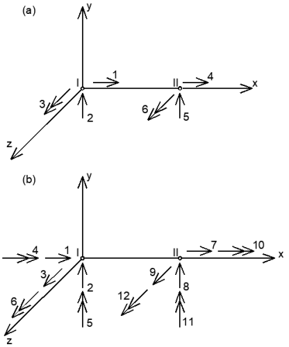
2.2. Bar Reference Axes and Movement Numbering
To express the stiffness coefficients, the translation and rotation movements are numbered according to the axes of the bar as follows:
Figure 1. Axes and movements of the bar: a) in the plane, b) in space.
2.3. Variable Section and Inertia Along the Bar
The elastic constants of a straight bar of variable section, of length L, are defined from the values of the area of its section along the bar and the moments of inertia and modulus of torsion, also along the bar.
To do this, the variation of these values is defined:
Variable Section AreaA(x)=A0ξ1(x)(2)
Variable Torque ModuleIt(x)=It0ξ2(x)(3)
Variable moment of inertia on the z-axisIz(x)=Iz0ξz3(x)(4)
Variable moment of inertia on the y-axisIy(x)=Iy0ξy3(x)(5)
A0, It0, Iz0, Iy0 being the reference values for the Section Area, the Torsion Modulus and the Moments of Inertia on the
z or
y axes respectively, (they are defined in a similar way to that established in Table 2.05-1 and Table 2.05-2 of
| [1] | Lahuerta, J. A. Formulario para el Proyecto de Estructuras. Dossat Madrid, 1.955. |
[1]
).
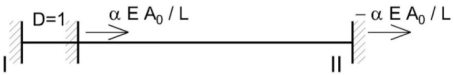
2.4. Longitudinal Stiffness of a Bar of Variable Section
The stiffness coefficients associated with a longitudinal deformation of a straight bar with the area of its variable section
A(x) = A0ξ1(x), are the actions produced at its ends by a unit longitudinal displacement applied to one of them (deduced from
| [2] | Lahuerta, J. A. Apuntes de Estructuras I, ETSAUN. |
[2]
(Form. 22.1)).
D =dx =dx =1(6)
To produce this displacement, it is necessary to apply a force N at the displaced end, and at the opposite end, a force N ́ = –N, of value:
N ==αA,being:α=(7)
These stiffness coefficients are part of the general expression of the Bar Stiffness Matrix in space established below (see
Figure 1b), and correspond to unit movements numbers 1 and 7. And on the plane with unitary movements 1 and 4.
Therefore, the coefficients of stiffness due to displacement 1, in space, are worth:
R1.1=α= AR7.1= -α= -A(8)
And the stiffness coefficients due to displacement 7 are worth:
R1.7= -α= -AR7.7=α= A(9)
On the plane: R1.1 = R4.4 = A R1.4 = R4.1 = - A
Figure 2. Stiffness coefficients for unitary longitudinal displacement at one end.
2.5. Torsional Rigidity in a Bar of Variable Section
The stiffness coefficients associated with an angular deformation along a straight bar with variable torsion modulus (Eq.
3) are the actions produced at its ends by a unit angular displacement applied to one of them.
D =dx =dx =1(10)
To produce this angular displacement, it is necessary to apply a torsional moment Tr to the rotated end, and to the opposite end a torsion moment Tr ́= –Tr, of value:
Tr==β,being:β=(11)
These stiffness coefficients are also part of the general expression of the Bar Stiffness Matrix in space (
Figure 1b), and correspond to unit turns numbers 4 and 10.
The stiffness coefficients due to such turns 4 and 10 are respectively valid:
R4.4 =β= TR10.4 = -β= -T(12)
R4.10 = -β= -TR10.10 =β= T(13)
Figure 3. Stiffness coefficients per unit longitudinal rotation at one end.
2.6. Deformation of a Bar of Variable Section
In order to determine the stiffness coefficients of the bar in the event of a rotation or translation at one of its ends, we first proceed to study the deformation of the bar.
In a simply supported isostatic bar of variable section the angles rotated in the extreme sections with respect to the y-axis, under the effect of the loads acting on the bar are:
| [1] | Lahuerta, J. A. Formulario para el Proyecto de Estructuras. Dossat Madrid, 1.955. |
[1]
2.05-7
́z=G ́z,being:G ́z=(14)
́ ́z=G´´z,being:G´´z=(15)
G ́z and G ́ ́ z are the load terms, which will be used to calculate the action values of equivalent ends of the variable section bar.
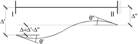
Figure 4. Bar with end twists and translations.
In the bar in
Figure 4, with end turns
θ', θ'' and end translations
, the value of the turns
θ’ and
θ’’ is:
| [1] | Lahuerta, J. A. Formulario para el Proyecto de Estructuras. Dossat Madrid, 1.955. |
[1]
2.05-7
θ´ = L/EIz(λ´zM´z-μzM´´z+G´z) +(16)
θ´´ = L/EIz(-μ´zM´z+λ´´zM´´z–G´´z) +(17)
Where λ´z, λ´´z, μz, are the "formal" or constants of the bar with respect to the z-axis, of value:
λ´z=λ´´z=μz=(18)
And to express the stiffness of the bar are defined:
| [1] | Lahuerta, J. A. Formulario para el Proyecto de Estructuras. Dossat Madrid, 1.955. |
[1]
2.05-8
ρ´z=ρ´z=ηz=(19)
The calculation of the stiffness coefficients of a bar that is produced, either by a unit rotation at its ends, or by linear displacement at its ends, can be obtained from the previous expressions where the Load Terms are null, since such coefficients are the value of the actions that produce a unit displacement and therefore there are no loads along the bar.
To calculate the stiffness coefficients, we will analyse two cases, those produced by a normal extreme unit rotation to the axis of the bar and those produced by a normal extreme unit displacement to the axis of the bar.
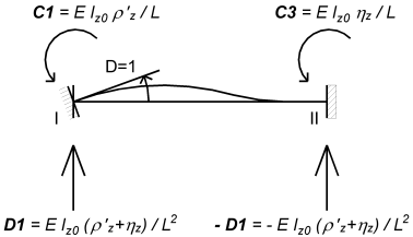
2.7. Unit rotational Stiffness at the End of the Bar with Variable Section in Space
In this case, represented in
Figure 1b, the unit turns in space correspond to movements 6 and 12 in the XY plane (z-axis rotation) and 5 and 11 in the XZ plane (y-axis rotation). See
Figure 1b.
In the XY plane (z-axis rotation), for turns 6 and 12 the values of the moments and normal forces at the ends of the bar as a consequence of a unit rotation at its end I, can be obtained from (
16 and
17) by doing:
Figure 5. Coefficients of stiffness per unit rotation at one end.
The values for the moment and force at the end I are:
MzI= E Iz0ρ´z/ L = C1VzI= - E Iz0(ηz+ρ´z) / L2= D1(21)
The values for the moment and force at the end II are:
MzII= E Iz0ηz/ L = C3VzII= E Iz0(ηz+ρ´z) / L2= - D1(22)
For the XZ plane you can proceed in a similar way.
The coefficients of stiffness due to such turns and movements are worth:
XY plane (z-axis turns):
R2.6= -R8.6= EIz0(ηz+ρ´z) /L2= Dz1R6.6= EIz0ρ´z/L= Cz1R12.6= EIz0ηz/L= Cz3(23)
R2.12= -R8.12= EIZ0(ηZ+ρ´´Z) /L2=Dz2R6.12= EIz0ηz/L=Cz3R12.12=EIz0ρ´´z/L= Cz2(24)
XZ plane (y-axis turns):
R3.5= -R9.5=EIy0(ηy+ρ´y) /L2= Dy1R5.5= EIy0ρ´y/L= Cy1R11.5= EIy0ηy/L= Cy3(25)
R3.11= -R9.11= - EIy0(ηy+ρ´´y) /L2= Dy2R5.11= EIy0ηy/L=Cy3R11.11= EIy0ρ´´y/L= Cy2(26)
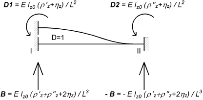
2.8. Transverse Displacement Stiffness at the Ends of a Bar of Variable Section in Space
To determine the stiffness coefficients associated with a displacement at the end of the bar normal to its axis, we start from the study of the bending deformation of the bar in section 2.6 above.
In this case, shown in
Figure 6, the unit displacements correspond to movements 3 and 9 in the XZ plane (z-axis displacement and y-axis rotation) and 2 and 8 in the XY plane (y-axis displacements
, and z-axis rotations). See
Figure 1b.
In the XY plane (z-axis rotation), for movements 2 and 8 the values of the moments and normal forces at the ends of the bar as a result of a unit displacement at its end I, can be obtained from (
16 and
17) by doing:
Figure 6. Coefficients of stiffness per unit displacement at one end.
The values for the moment and force at the end I are:
MzI= E Iz0(ρ´z+ηz) / L2= Dz1(28)
VzI= E Iz0(ρ´z+ρ´´z+2ηz) / L3= Bz(29)
The values for the moment and force at the end II are:
MzII= E Iz0(ρ´´z+ηz) / L2= Dz2(30)
VzII= - E Iz0(ρ´z+ρ´´z+2ηz) / L3= - Bz(31)
In the XZ plane you can proceed in a similar way.
The coefficients of stiffness due to such movements are worth:
XY plane (z-axis turns):
R2.2= - R8.2= E Iz0(ρ´z+ρ´´z+2ηz) / L3=BzR6.2= E Iz0(ρ´z+ηz) / L2= Dz1R12.2= E Iz0(ρ´´z+ηz) / L2= Dz2(32)
R8.8= -R2.8= EIy0(ρ´z+ρ´´z+2ηz) /L3=BzR6.8= -E Iz0(ρ´z+ηz) / L2= - Dz1R12.8= - E Iz0(ρ´´z+ηz) / L2= - Dz2(33)
XZ plane (y-axis turns):
R3.3= -R9.3= EIy0(ρ´y+ρ´´y+2ηy) /L3= ByR5.3= -Dy1R11.3= -Dy2(34)
R9.9= -R3.9= EIy0(ρ´y+ρ´´y+2ηy) /L3= ByR5.9= - Dy1R11.9= - Dy2(35)
3. The Stiffness Matrix of the Variable Section Bar
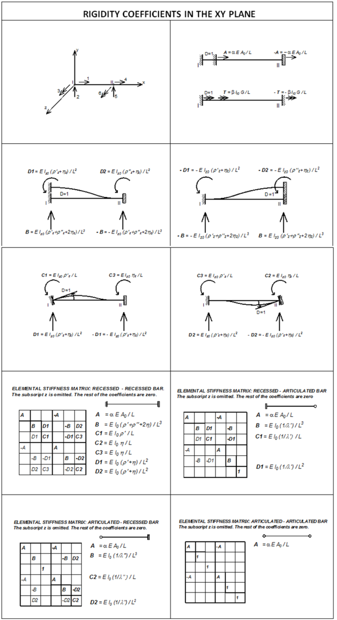
3.1. Stiffness Matrix of a Bar of Variable Section in the Plane
As stated in Section 2.1, the Matrix
Rb of Stiffness of the ends of a bar in the plane has a size of 6x6 and expresses the interrelation between the vector
Ab of equivalent actions of the end with the
vector Db of movements of the end of the bar (Eq.
1)
This equation refers to the proper axes of the bar, with three possible movements (two linear and one rotation) for each end of the bar (
Figure 1a), and 3 possible movements (2 linear and 1 rotation).
Figure 7. Stiffness matrix of a bar of variable section in the plane.
Adopting the agreement of signs expressed in
Figure 1a, the stiffness matrix R
b of the bar in the plane according to the parameters defined above will be that expressed in
Figure 7 for the four cases of bars: recessed – recessed, recessed – articulated, articulated – recessed and articulated – articulated:
(The subscript “y” has been removed for convenience for Iz0, ρz', ρz" y ηz)
The Stiffness Matrix R is square and symmetrical and its coefficients are indicated in the table, being:
A is the area with
A0 reference value and
ξ1(x) the law of variation, (Eq.
2),
I the moment of inertia with
I0 reference value (Eq.
4), and
ξ3(x) its law of variation,
α, λ´, λ´´ and μ, the formal ones (Eqs.
7,
18) and
ρ´, ρ´´ and η, rigidities (Ec.
19).
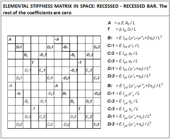
3.2. Stiffness Matrix of a Bar of Variable Section in Space
Adopting the convention of signs expressed in
Figure 1b, the Stiffness Matrix of a bar in space will be a square and symmetrical matrix of size 12 x 12, which corresponds to six movements for each knot of the same, three linear according to the axes and three rotations around these axes.
The elemental stiffness matrix for the bar in space according to the axis system in
Figure 1b) is as follows:
Figure 8. Stiffness matrix of a bar of variable section in space.
3.3. Actions at the Ends of the Variable Section Bar
To determine the vector A
The equivalent system of loads applied at the ends of the bars can then be calculated from the values of the reactions, with the opposite sign.
Therefore, the problem of determining the system of actions at the end of the bar is reduced to the calculation of the reactions of the real load system in the bar supposed to be embedded or articulated at one of its ends.
These section bar end actions or variable stiffness are different from those obtained for a section bar and constant stiffness.
Recessed – recessed bars.
Reactions can be determined from the Equations
(16 and 17), doing:
θ'y =θ"y =Δ =0:M'y= -ρ'yG’y+ηyG’'yM"y= -ηyG'y+ρ"yG"y(36)
Recessed – articulated bars.
M'y= - (1/λ'y)G’yM"y= 0(37)
Articulated – recessed bars.
M'y= 0M"y= (1/λ”y)G”y(38)
In this expression
G'y,
G"y are the terms of load defined in Section 2.6 (Ec.
14, 15)
Shear stresses are deduced from isostatic moments from extremes.
4. Example 1 for Application of the Method
To illustrate, step by step, the development of the described method, the following calculation example is proposed
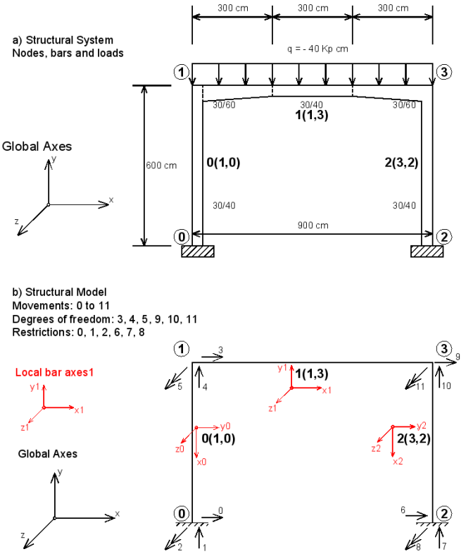
It is a flat portico, represented in
Figure 9, composed of a poster lintel and two supports that are supposed to be embedded in its base.
The portico is designed with H-25 reinforced concrete with AEH-500 and its geometric data and the loads that act are represented in
Figure 9. The units used are Kp and cm.
Figure 9. The case of a simple portico. Structural System and Structural Model.
4.1. Structural Model
Numbering of bars and knots.
The structural model that represents this idealized and discretized structure, (
Figure 9b), is composed of 4 nodes (numbered from 0 to 3), three bars (numbered from 0 to 2) whose initial and final nodes are (1,0), (1,3) and (3,2) respectively. The bars are connected to each other at their ends, which are the nodes of the structural model, the only points considered in the relationship between actions and movements or stiffness equation.
Support of the bars.
The support system of the bars is formed by the movement restrictions of their ends, and is as follows: Knots 0 and 2 are knots restricted in all their movements and knots 1 and 3 are free with rigid connections between their bars.
Numbering of knot movements.
The movements of the knots are numbered in the order shown in
Figure 9b. Those corresponding to nodes 0 and 2 (0, 1, 2, 6, 7 and 8) are null (restricted). Those corresponding to nodes 1 and 3 (3, 4, 5, 9, 10, 11) are degrees of freedom (DOF).
Section of the bars and terms of area variation and inertia along the bars.
The terms of variation of the section and inertia of bars
A(x) and
Iy(x), defined in Section 2.3 (Eqs.
2, 4) are as follows:
Reference values:
Iy0= 30 x 403/12 = 160.000cm4
1-0 and 3-2 bars:
They are of constant cross-section equal to the reference value:
The variation terms are:
ξ1(x) =ξ3y(x) = 1, con lo cual las formales (7, 18 y 19) son:
αz= 1λ'y =λ"y = 1/3μy = 1/6ρ'y =ρ"y =4ηy = 2
Barra 1-3:
It has a variable section due to the gussets and is divided into three sections, 1/3 of the length of the span.
The variation terms are:
Tramo(0,300):ξ1(x) = 1,5-x/600ξ3(x) = (1/40^3) * (60- 20x/300)3
Tramo (300,600):ξ1(x) = 1ξ3(x) = 1
Tramo (600,900):ξ1(x) = 1 + (x-600) / 600ξ3(x) = (1/40^3) * (40+ 20(x-600) /300)3
α== 1.14422
λ´= (403/9003) * () = 0,2156
λ´´= (403/9003) * () = 0,2156
μ= (403/9003) * () = 0,1363
ρ´y==0,2156/0,0279 = 7,7249
ρ´´y==0,2156/0,0279 = 7,7249
ηy==0,1363/0,0279 = 4,8828
4.2. Equivalent System of Actions Acting on the Ends of the Bars
The system of actions acting in the structural system is formed by the distributed load
q, which must be replaced by an equivalent system of loads acting at the ends of the bars to maintain the discrete character of these structural elements. The equivalent system is composed of the reactions:
M', M", V', V", only of bar 1 (nodes 1 to 3) produced by the charge
q = - 40 (negative for in the opposite direction to the y-axis) acting at nodes 1 and 3. The values of
M'y, M"y are determined as follows (Ec.
36 and
37):
Bar1-3, with: Mis, y(x) = q x (L-x)/2, the charge terms G' and G" are:
G´y== - 40 /(2*9002)*(403()) = - 1.103.772
G´´y== - 40 / (2*9002) * (403()) = - 1.103.772
The reactions M', M', V', V", taking into account the direction of the charge in and worth:
M'y=-(-ρ'yG’y+ηyG’'y) =- 3.137.025cmKpV'= - 18.000Kp
M"y = -(-ηyG'y +ρ"yG"y) = 3.137.025 cmKpV"= - 18.000 Kp
The system of equivalent actions (reactions) for bar 1-3 can be represented by the vector A,
A=
The equivalent actions produced by bars 0 (1-0) and 2 (3-2) are null and void as there are no charges acting on them.
In global coordinates, the equivalent actions of the 4 nodes are:
A=
4.3. Calculation of the Coefficients of the Stiffness Matrix
The elementary stiffness matrices of each bar are calculated according to
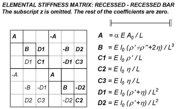
Figure 7 for recessed bars – recessed in their local axes:
Figure 10. Elemental Stiffness Matrix: Recessed and Recessed bar.
These matrices are then transferred to global axes by means of the transformation matrix, and once on global axes the global rigidity matrix of the structure is assembled.
The resulting matrices in this process are the following:
For Bar 0.
A0= 1.200 cm2, I0= 160.000 cm4, L = 600 cm, E = 310.000 k/cm2,α= 1,ρ'y =ρ"y =4,ηy = 2
B = E I0(ρ´+ρ´´+2η) / L3=2755.5
D1 = EI0(η+ρ´) /L2=826666.6
D2 = EI0(η+ρ´´) /L2=826666.6
Table 1. Elemental Stiffness Matrix on bar shafts (MR_elem_0).
620000 | 0 | 0 | -620000 | 0 | 0 |
0 | 2755.5 | 826666.6 | 0 | -2755.5 | 826666.6 |
0 | 826666.6 | 330666666.6 | 0 | -826666.6 | 165333333.3 |
-620000 | 0 | 0 | 620000 | 0 | 0 |
0 | -2755.5 | -826666.6 | 0 | 2755.5 | -826666.6 |
0 | 826666.6 | 165333333.3 | 0 | -826666.6 | 330666666.6 |
Table 2. Transformation Matrix (T_0).
0 | -1 | 0 | 0 | 0 | 0 |
1 | 0 | 0 | 0 | 0 | 0 |
0 | 0 | 1 | 0 | 0 | 0 |
0 | 0 | 0 | 0 | -1 | 0 |
0 | 0 | 0 | 1 | 0 | 0 |
0 | 0 | 0 | 0 | 0 | 1 |
Table 3. Matrix of the bar on global axes (K_global_0): (K_global_0) =(T_0T) x (MR_elem_0) x (T_0).
2755.5 | 0 | 826666.6 | -2755.5 | 0 | 826666.6 |
0 | 620000 | 0 | 0 | -620000 | 0 |
826666.6 | 0 | 330666666.6 | -826666 | 0 | 165333333.3 |
-2755.5 | 0 | -826666.6 | 2755.5 | 0 | -826666.6 |
0 | -620000 | 0 | 0 | 620000 | 0 |
826666.6 | 0 | 165333333.3 | -826666 | 0 | 330666666.6 |
For Bar 1.
A0 = 1.200 cm2, I0 = 160.000 cm4, L = 900 cm, E = 310.000 k/cm2, α = 1.1442, ρ'y = ρ"y =7.72763, ηy = 4.8827. (Some value may differ somewhat by the calculation algorithm)
B = E I0(ρ´+ρ´´+2η) / L3=1715.9
D1 = EI0(η+ρ´) /L2=772192.4
D2= EI0(η+ρ´´) /L2= 772192.4
Table 4. Elemental Stiffness Matrix on bar shafts (MR_elem_1).
472939.9 | 0 | 0 | -472939 | 0 | 0 |
0 | 1715.9 | 772192.4 | 0 | -1715.9 | 772192.4 |
0 | 772192.4 | 425878491.3 | 0 | -772192 | 269094744.6 |
-472939 | 0 | 0 | 472939 | 0 | 0 |
0 | -1715.9 | -772192.4 | 0 | 1715.9 | -772192.4 |
0 | 772192.4 | 269094744.6 | 0 | -772192 | 425878491.3 |
Table 5. Transformation Matrix (T_1).
1 | 0 | 0 | 0 | 0 | 0 |
0 | 1 | 0 | 0 | 0 | 0 |
0 | 0 | 1 | 0 | 0 | 0 |
0 | 0 | 0 | 1 | 0 | 0 |
0 | 0 | 0 | 0 | 1 | 0 |
0 | 0 | 0 | 0 | 0 | 1 |
Table 6. Matrix of the bar on global axes (K_global_1): (K_global_1) =(T_1T) x (MR_elem_1) x (T_1).
472939.9 | 0 | 0 | -472939 | 0 | 0 |
0 | 1715.9 | 772192.4 | 0 | -1715.9 | 772192.4 |
0 | 772192.4 | 425878491.3 | 0 | -772192 | 269094744.6 |
-472939 | 0 | 0 | 472939.9 | 0 | 0 |
0 | -1715.9 | -772192.4 | 0 | 1715.9 | -772192.4 |
0 | 772192.4 | 269094744.6 | 0 | -772192 | 425878491.3 |
For Bar 2. (It's the same as for bar 0)
A0= 1.200 cm2, I0= 160.000 cm4, L = 600 cm, E = 310.000 k/cm2,α= 1,ρ'y =ρ"y =4,ηy = 2
B = E I0(ρ´+ρ´´+2η) / L3=2755.5
D1 = EI0(η+ρ´) /L2=826666.6
D2 = EI0(η+ρ´´) /L2= 826666.6
Table 7. Elemental Stiffness Matrix on bar shafts (MR_elem_2).
620000 | 0 | 0 | -620000 | 0 | 0 |
0 | 2755.5 | 826666.6 | 0 | -2755.5 | 826666.6 |
0 | 826666.6 | 330666666.6 | 0 | -826666.6 | 165333333.3 |
-620000 | 0 | 0 | 620000 | 0 | 0 |
0 | -2755.5 | -826666.6 | 0 | 2755.5 | -826666.6 |
0 | 826666.6 | 165333333.3 | 0 | -826666.6 | 330666666.6 |
Table 8. Transformation Matrix (T_2).
0 | -1 | 0 | 0 | 0 | 0 |
1 | 0 | 0 | 0 | 0 | 0 |
0 | 0 | 1 | 0 | 0 | 0 |
0 | 0 | 0 | 0 | -1 | 0 |
0 | 0 | 0 | 1 | 0 | 0 |
0 | 0 | 0 | 0 | 0 | 1 |
Table 9. Matrix of the bar on global axes (K_global_2): (K_global_2) =(T_2T) x (MR_elem_2) x (T_2).
2755.5 | 0 | 826666.6 | -2755.5 | 0 | 826666.6 |
0 | 620000 | 0 | 0 | -620000 | 0 |
826666.6 | 0 | 330666666.6 | -826666 | 0 | 165333333.3 |
-2755.5 | 0 | -826666.6 | 2755.5 | 0 | -826666.6 |
0 | -620000 | 0 | 0 | 620000 | 0 |
826666.6 | 0 | 165333333.3 | -826666 | 0 | 330666666.6 |
4.4. Global Stiffness Matrix and Stiffness Equation
The coefficients that make up the Global Stiffness Matrix are obtained by adding those of the elementary bar matrices in global coordinates, in the position that corresponds to them according to the numbering of movements.
These elementary matrices in global coordinates have been calculated in section 4.3 above.
Once the Global Stiffness Matrix has been assembled in this way, it is necessary to apply the boundary conditions to it by cancelling the equations that correspond to the restricted movements (which are movements 0, 1, 2, 6, 7 and 8) equalizing their coefficients to 0 minus that of the main diagonal to which the value 1 is given.
The 12x12
[[1, 0, 0, 0, 0, 0, 0, 0, 0, 0, 0, 0]
[0, 1, 0, 0, 0, 0, 0, 0, 0, 0, 0, 0]
[0, 0, 1, 0, 0, 0, 0, 0, 0, 0, 0, 0]
[0, 0, 0, 475695, 0, 826666, 0, 0, 0, -472939, 0, 0]
[0, 0, 0, 0, 621715, 772192, 0, 0, 0, 0, -1715, 772192]
[0, 0, 0, 826666, 772192, 756545158, 0, 0, 0, 0, -772192, 269094744]
[0, 0, 0, 0, 0, 0, 1, 0, 0, 0, 0, 0]
[0, 0, 0, 0, 0, 0, 0, 1, 0, 0, 0, 0]
[0, 0, 0, 0, 0, 0, 0, 0, 1, 0, 0, 0]
[0, 0, 0, -472939, 0, 0, 0, 0, 0, 475695, 0, 826666]
[0, 0, 0, 0, -1715, -772192, 0, 0, 0, 0, 621715, -772192]
[0, 0, 0, 0, 772192, 269094744, 0, 0, 0, 826666, -772192, 756545158]]
And the vector of Global Forces is (F_global_total):
[[0], [0], [0], [0], [-18000], [-3136332], [0], [0], [0], [0], [-17999], [3136332]]
The stiffness equation of the model is:
(K_global_total) x D = (F_global_total)
Once the system is solved, the vector D is obtained, whose value is:
[[0], [0], [0], [0.005615197581263467], [-0.02903225806451541], [-0.006443680670371993], [0], [0], [0], [-0.005615197580875675], [-0.02903225806451604], [0.006443680670370919]]
From this vector the displacements that correspond to bar 1, which are the only non-zero ones, coincide with those of the local coordinates of bar 1:
Table 10. Vector (desp_local_1).
0.005615197581263467 |
-0.02903225806451541 |
-0.006443680670371993 |
-0.005615197580875675 |
-0.02903225806451604 |
0.006443680670370919 |
Table 11. Elemental Stiffness Matrix on bar shafts (MR_elem_1).
472939.9 | 0 | 0 | -472939 | 0 | 0 |
0 | 1715.9 | 772192.4 | 0 | -1715.9 | 772192.4 |
0 | 772192.4 | 425878491.3 | 0 | -772192 | 269094744.6 |
-472939 | 0 | 0 | 472939 | 0 | 0 |
0 | -1715.9 | -772192.4 | 0 | 1715.9 | -772192.4 |
0 | 772192.4 | 269094744.6 | 0 | -772192 | 425878491.3 |
Multiplying (MR_elem_1) x (desp_local_1) yields the values of the internal forces, which added to the equivalent actions of the bar (AC_equiv_1) gives the final actions at the ends of the bar.
4.5. Calculation of Actions at the Ends of the Bars
From the above, the actions at the ends of bar 1 (nodes 1,3) are as follows:
A1-3 = (MR_elem_1) x (desp_local_1) + (AC_equiv_1) =N' = -5311= -5.3 t
V’ = -18000 = -18 t
M’ = -2126068 = -21.2mt
N" = 5311 = -5.3 t
V” = -18000 = -18 t
M" = 2126068 = 21.2mt
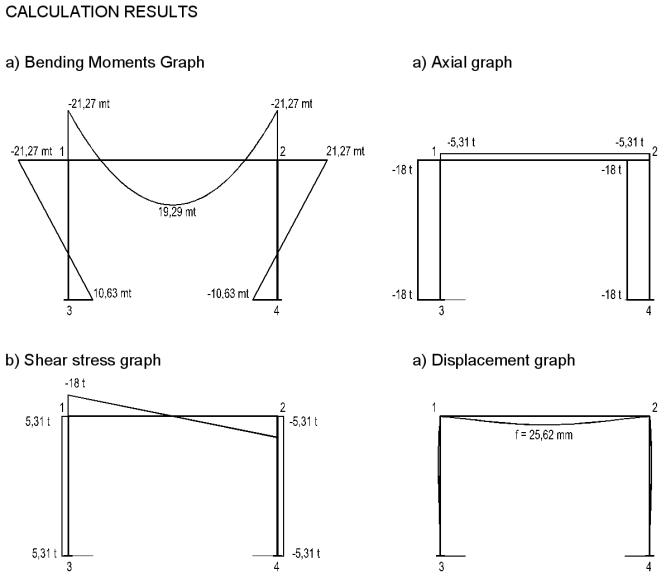
4.6. Calculation Results
The stresses resulting from the calculation are shown below graphically by changing the units to m and t (meters and tons). These stresses are used to calculate the necessary reinforcements in the case of reinforced concrete, for which the method found in Annex 7 of
| [4] | EHE-08. Ministerio de Fomento. Spain. |
[4]
can be used.
Figure 11. Calculation Results.
5. Conclusion
By means of this approach to the Stiffness Matrix for bars of variable section, any structure of straight bars with variable section can be calculated by the Stiffness Matrix Method.
The matrix equations that result is of the same size as those used for bars of constant section, although the coefficients of the matrix are different and must be obtained by integration along the bar.
The same happens with the equivalent actions of the end of the bar, which also have to be calculated by integration.
Because obtaining the Coefficients of the Stiffness Matrix by integration along the bar can be laborious when the variation of its mechanical constants or the distribution of moments becomes complicated, numerical integration is advantageous.
To this end, Simpson's rule obtains sufficient precision, with not too many intervals.
In isotropic materials, the direct application of the method for variable section bars can be carried out directly from their geometry without the need to make hypotheses about the behaviour of the material as when it is non-isotropic.
This happens in the example of section 4 and is also the case of steel profiles that have reinforcements in some areas. For example, gussets or reinforcements in bars that increase their rigidity in the reinforced areas, as can happen in metal columns when certain types of semi-rigid joints are used to thicken them and have a lot of influence on the seismic calculation.
In the case of non-isotropic materials, such as reinforced concrete in a cracked state or mixed beams, it is necessary to establish hypotheses that define the laws of variation of the mechanical constants of the bars.
There are numerous structural systems where the variable stiffness of the bars can be significant, so applying the method can be useful and be the subject of new studies.
This study is complemented by a Python program whose source code is provided so that it can be reviewed, modified and improved by any interested party.
Abbreviations
A | Area |
Ab | Bar End Equivalent Actions |
D | Longitudinal Displacement |
Db | Bar End Movements |
E | Warp Module |
F | Action |
G', G" | Charging Terms |
I | Moment of Inertia |
It | Torque Modulus |
K | Coefficient |
L | Longitude |
M | Bending Moment |
N | Normal Strength |
Rb | Stiffness Matrix |
T | Torsor Moment |
U | Mechanical Capability |
V | Shear Stress |
W | Rugged Module |
a | Distance. Arrow |
b | Width |
d | Useful Song |
e | Eccentricity |
f | Resistance |
g | Permanent Load Spread |
h | Canto Total |
i | Turning Radius |
k | Coefficient |
l | Length, Light |
m | Bending moment per unit length |
w | Arrow |
α (Alpha) | Angle, Coefficient |
β (Beta) | Angle, Coefficient |
γ (Gamma) | Weighting Coefficient |
ε (Epsilon) | Relative Deformation |
η (Eta) | Stiffness Coefficient |
θ (Theta) | Angle |
λ (Lambda) | Formal Bar |
μ (Mu) | Formal Bar |
ν (Nu) | Relative Normal Effort |
ξ (xi) | Coefficient of Variation |
ρ (Rho) | Geometric Amount |
ρ', ρ" | Stiffness Coefficients |
σ (Sigma) | Tension. Tangential Tension |
φ (Fee) | Coefficient |
ψ (Psi) | Coefficient |
ω (Omega) | Mechanical Amount |
Acknowledgments
In this study I have intended, above all, to honoting the memory of Professor Don Javier Lahuerta Vagas, who died in 2009, with whom I shared many hours commenting on the topics presented here and who helped me with his valuable advice to develop many of the ideas raised here.
Much of what is developed here is based on his research work.
Secondly, I must say that this work is a research work, which may not be free of errors, but which we want to disseminate so that it can be used and improved by anyone interested in the subject.
Finally, I must point out that many of the programming algorithms in Python to analyze specific examples have been developed with the collaboration of the AI program "Copilot" integrated in W11 Edge to which I thank for its help.
Author Contributions
Angel Ibáñez Ceba is the sole author. The author read and approved the final manuscript.
Conflicts of Interest
The authors declare no conflicts of interest.
References
| [1] |
Lahuerta, J. A. Formulario para el Proyecto de Estructuras. Dossat Madrid, 1.955.
|
| [2] |
Lahuerta, J. A. Apuntes de Estructuras I, ETSAUN.
|
| [3] |
Lahuerta, J. A. Estructuras de edificación, ETSAUN 1.985.
|
| [4] |
EHE-08. Ministerio de Fomento. Spain.
|
| [5] |
Xu, Leiping&Hou, Pengfei& Han, Bing. (2016). Stiffness Matrix of Timoshenko Beam Elemen twith Arbitrary Variable Section. 2991/mmebc-16.2016.405.
|
| [6] |
Mancuso, Caitlin& Bartlett, F. (2017). ACI 318-14 Criteria for Computing Instantaneous Deflections. ACI Structural Journal. 114.
https://doi.org/10.14359/51689726
|
| [7] |
Celigüeta, J. Tomás. Diseño de Estructuras. Método de rigidez para cálculo de estructuras reticulares. Tecnun Universidad de Navarra 2016.
|
| [8] |
Celigüeta, J. Tomás. Curso de Análisis Estructural. Tecnun Universidad de Navarra 2022.
|
| [9] |
Blanco E., Cervera M. y Suárez B. Análisis Matricial de Estructural. CIMNE 2015.
|
| [10] |
Sánchez Molina, D. y González R. Cálculo de elementos estructurales. UPC GRAU 2011.
|
Cite This Article
-
-
@article{10.11648/j.ijmsa.20251401.12,
  author = {Angel Ibáñez Ceba},
  title = {Stiffness Matrix for Bars with Variable Section or Inertia
},
  journal = {International Journal of Materials Science and Applications},
  volume = {14},
  number = {1},
  pages = {13-28},
  doi = {10.11648/j.ijmsa.20251401.12},
  url = {https://doi.org/10.11648/j.ijmsa.20251401.12},
  eprint = {https://article.sciencepublishinggroup.com/pdf/10.11648.j.ijmsa.20251401.12},
  abstract = {The matrix calculation by the Stiffness Matrix Method for structures composed of straight bars is normally performed considering the bars with constant section and inertia, and when the bars are of variable section, intermediate nodes are introduced, significantly increasing the size of the Stiffness Matrix. In this work, a generalization of the Stiffness Matrix Method for structures with bars of variable section and/or inertia is proposed, introducing adequate matrix coefficients for the calculation with bars with variable section and/or inertia, maintaining the number of nodes of the structure and therefore without increasing the size of the Stiffness Matrix. In practice, many structural systems are made up of bars of variable section or inertia, such as cartelized bars, cracked reinforced concrete bars, steel bars with semi-rigid joints or mixed concrete and steel bars. In all these cases, the result of the calculation when considering the constant section is, in general, approximate and must be interpreted taking into account the simplification introduced by the calculation, for example, in the calculation of deflections or deformations for concrete bars in a cracked state, which is the normal state in which they are found. In this case, the consideration of bars with a constant section yields results that are far from reality. And in other cases, something similar happens. Therefore, the generalization of the Stiffness Matrix Method for structures with variable section and/or inertia bars is really a refinement of the Stiffness Matrix calculation method that can be useful in many cases, and also provide results more in line with reality
},
 year = {2025}
}
 Copy
|
Copy
|
 Download
-
TY  - JOUR
T1  - Stiffness Matrix for Bars with Variable Section or Inertia

AU  - Angel Ibáñez Ceba
Y1  - 2025/03/18
PY  - 2025
N1  - https://doi.org/10.11648/j.ijmsa.20251401.12
DO  - 10.11648/j.ijmsa.20251401.12
T2  - International Journal of Materials Science and Applications
JF  - International Journal of Materials Science and Applications
JO  - International Journal of Materials Science and Applications
SP  - 13
EP  - 28
PB  - Science Publishing Group
SN  - 2327-2643
UR  - https://doi.org/10.11648/j.ijmsa.20251401.12
AB  - The matrix calculation by the Stiffness Matrix Method for structures composed of straight bars is normally performed considering the bars with constant section and inertia, and when the bars are of variable section, intermediate nodes are introduced, significantly increasing the size of the Stiffness Matrix. In this work, a generalization of the Stiffness Matrix Method for structures with bars of variable section and/or inertia is proposed, introducing adequate matrix coefficients for the calculation with bars with variable section and/or inertia, maintaining the number of nodes of the structure and therefore without increasing the size of the Stiffness Matrix. In practice, many structural systems are made up of bars of variable section or inertia, such as cartelized bars, cracked reinforced concrete bars, steel bars with semi-rigid joints or mixed concrete and steel bars. In all these cases, the result of the calculation when considering the constant section is, in general, approximate and must be interpreted taking into account the simplification introduced by the calculation, for example, in the calculation of deflections or deformations for concrete bars in a cracked state, which is the normal state in which they are found. In this case, the consideration of bars with a constant section yields results that are far from reality. And in other cases, something similar happens. Therefore, the generalization of the Stiffness Matrix Method for structures with variable section and/or inertia bars is really a refinement of the Stiffness Matrix calculation method that can be useful in many cases, and also provide results more in line with reality

VL  - 14
IS  - 1
ER  -
Copy
|
Download