Understanding climate variability and monitoring time-series trends of temperature and rainfall is crucial for the sustainable development of our planet. This study utilized historical data from the Global Historical Climatology Network-Monthly (GHCN-M) provided by the National Centers for Environmental Information (NCEI) to analyze the temperature and rainfall data from 2015 to 2022. The analysis was conducted using Python 3.1.1 on Anaconda Jupyter Notebook and the package matplotlib 3.2.1 was used for data visualization. The results revealed a pattern of maximum rainfall between March to May for the years 2020, 2021, and 2022, while for the years 2017, 2018, and 2019, the maximum rainfall was recorded in October, December, and November. Additionally, the annual maximum rainfalls were recorded in the years 2020 and 2022, and the annual maximum temperatures for all study years were recorded in January, February, and March months. On the other hand, the annual minimum temperatures for all study years occurred in June, July, August, and September months. Similarly, annual average temperatures were recorded in January, February, and March months. This study emphasizes the importance of monitoring climate change and its impacts on our planet. By understanding climate variability and time-series trends, we can better prepare for the future and work towards a sustainable world.
This is an Open Access article, distributed under the terms of the Creative Commons Attribution 4.0 International License (http://creativecommons.org/licenses/by/4.0/), which permits unrestricted use, distribution and reproduction in any medium or format, provided the original work is properly cited.
Time Series Analysis, Precipitation, Temperature, Rainfall, Jupyter Notebook, Matplotlib
1. Introduction
Climate change represents a significant addition to the spectrum of environmental health hazards that humankind faces. Its global scale generates unfamiliarity, though most of its health impacts are increases or decreases in familiar effects of climatic variation on human biology and health
[1]
McMichael, A. J., et al., eds. Climate change and human health Risks and Responses. World Health Organization Geneva. 2003.
[1]
. Climate variability and change have become major environmental challenges of the 21st century, threatening both food security and sustainable development, as well as the totality of human existence
[2]
Belay, F. E., et al., Spatio-Temporal Variability and Time Series Trends of Monthly and Seasonal Rainfall Over Northwestern Ethiopia.. Global Journal of Environmental Research, 2020. 14(2): p. 45-54.
[2]
. In addition according to Belay, F. E., et al., climate change is a global concern as it severely affects the livelihoods of the world community in general and agricultural production as well as food security of rural community in particular.
Modeling the variations of surface temperature and making dependable forecasts underlie the foundation of sound environmental policies
[3]
Ye L. M., G. X., et al., Time-series modeling and prediction of global monthly absolute temperature for environmental decision making.. Adv. Atmos. Sci.,, 2013. 30(2): p. 382-396.
[3]
. Especially, time series analysis and modeling of mean monthly temperature and total monthly precipitation are two most important climatic variables that easily obtained from weather station records
[4]
Mulomba, P. M. and C. González-García, Time Series Analysis of Climatic Variables in Peninsular Spain. Trends and Forecasting Models for Data between 20th and 21st Centuries. Climate, 2021. 9(119).
[4]
. However, time series (TS) analysis is a frequent and challenging topic of both today and future research in remote sensing (RS). But these problems are solved using technology like global earth observation (EO) programs that provide extensive temperature and precipitation data archives dating back several years or even more decades (e.g., Sentinel, Landsat etc.). On other hand on a country-wide scale, aerial images, LiDAR (Light Detection and Ranging) and photogrammetric point clouds are acquired in two to three year cycles
[5]
Markéta, P., et al., E-TRAINEE: OPEN E-LEARNING COURSE ON TIME SERIES ANALYSIS IN REMOTE SENSING. The International Archives of the Photogrammetry, Remote Sensing and Spatial Information Sciences,, 2023. XLVIII-1/W2-2023.
[5]
. Importantly, time series analysis has always been an important topic in remote sensing it is applied by open access to archives of Earth Observation missions, periodically acquired nation-wide aerial imagery and LiDAR point clouds, and various research datasets, together with open tools for time series data processing, it have brought new possibilities in Remote Sensing research but also challenges in education
[5]
Markéta, P., et al., E-TRAINEE: OPEN E-LEARNING COURSE ON TIME SERIES ANALYSIS IN REMOTE SENSING. The International Archives of the Photogrammetry, Remote Sensing and Spatial Information Sciences,, 2023. XLVIII-1/W2-2023.
[5]
. With an increasingly supported and accepted of these open data policy free access to these data sources has become a well - recognized practice. Specific sites are monitored on a regular basis (weekly, monthly, yearly) for diverse research purposes.
Time series analyses are used frequently to analyze exposures associated with short-term variability of climate. Time series analyses can take account of cyclical patterns, such as seasonal patterns, when evaluating longitudinal trends in disease rates in one geographically defined population
[1]
McMichael, A. J., et al., eds. Climate change and human health Risks and Responses. World Health Organization Geneva. 2003.
[1]
. Seasonal patterns may be due to the seasonality of climate or to other factors, such as the school year
[1]
McMichael, A. J., et al., eds. Climate change and human health Risks and Responses. World Health Organization Geneva. 2003.
[1]
.
Two generally used approaches to time series analyses are generalized additive models (GAM) and generalized estimating equations (GEE). The generalized additive model entails the application of a series of semi-parametric Poisson models that use smoothing functions to capture long-term patterns and seasonal trends from data. However, no a priori smoothing is performed for the time series. Instead, the GEE model allows for the removal of long-term patterns in the data by adjusting for over dispersion and autocorrelation. Autocorrelation needs to be controlled for in time series data of weather measurements because today’s weather is correlated with weather on the previous and subsequent days
[1]
McMichael, A. J., et al., eds. Climate change and human health Risks and Responses. World Health Organization Geneva. 2003.
[1]
.
For example a study by Hay et al. demonstrates one approach for looking at longer-term variability (48). The authors used spectral analysis to investigate periodicity in both climate and epidemiological time series data of dengue hemorrhagic fever (DHF) in Bangkok, Thailand. DHF exhibits strong seasonality, with peak incidences in Bangkok occurring during the months of July, August and September. This seasonality has been attributed to temperature variations. Spectral analysis (or Fourier analysis) uses stationary sinusoidal functions to deconstruct time series into separate periodic components. A broad band of two to four year periodic components was identified as well as a large seasonal periodicity. One limitation of this method is that it is applicable only for stationary time series in which the periodic components do not change
[1]
McMichael, A. J., et al., eds. Climate change and human health Risks and Responses. World Health Organization Geneva. 2003.
[1]
. Specifically, Rainfall forecasting is one of the most crucial functions of meteorological departments for all countries. According to Waqas M. et al forecasting rainfall helps to prevent flooding to reduce loss of lives and property and it facilitates the management of water resources
[6]
Waqas, M., et al., Potential of Artificial Intelligence-Based Techniques forRainfall Forecasting in Thailand. A Comprehensive Review. Water 2023. 15(2979).
[6]
.
In other case, temperature data are usually given as monthly means in an equally spaced time series. Instrumental records used in computing these mean values globally have only been available for the past ∼150 years
[7]
Jones, P. D. and A. Moberg, 2003: Hemispheric and large-scale surface air temperature variations:. An extensive revision and an update to 2001. Climate, 2001. 16: p. 206-223.
[7]
. Many efforts have been made in the statistical modeling of temperature variations using these records (e.g.
[8]
Hansen, J. M., et al., Global temperature change.. Proc. National Academy of Sciences USA,, 2006. 103: p. 14288-14293.
[9]
Rahmstorf, A. S., et al., Recent climate observations compared to projections.. Science,, 2007. 316.
[8, 9]
). Among them, the univariate time-series models have gained relative popularity in recent years, partly due to the complexity of mainstream climate models, which are strongly constrained by the current knowledge of the physical climate system
[10]
IPCC, Detection of climate change and attribution of causes. in Climate Change 2001: The Scientific Basis. Contribution of Working Group I to the Third Assessment Report of the Intergovernmental Panel on Climate Change, J. T. Houghton et al., Eds., Cambridge University Press. 2001. p. 44.
[10]
. One subcategory of the univariate models, namely the structural time-series models
[11]
Lee, H. J. and K.-T. Sohn, Prediction of monthly mean surface air temperature in a region of China.. Adv. Atmos. Sci.,, 2007. 24: p. 503-508.
[11]
, has become quite popular due to its trend-detecting capability
[3]
Ye L. M., G. X., et al., Time-series modeling and prediction of global monthly absolute temperature for environmental decision making.. Adv. Atmos. Sci.,, 2013. 30(2): p. 382-396.
[3]
. Many time series forecasting methods are based on the analysis of historical data. They assume that past patterns in the data can be used to forecast future events
[12]
Murat, M., et al., Forecasting Daily Meteorological Time Series Using ARIMA and Regression Models. Int. Agrophys., 2018. 32.
[12]
.
This study was conducted to answer the following questions using time series analysis method 1) what is the monthly minimum temperature between 2015 and 2022 years using time series analysis? 2) What is the monthly maximum temperature between 2015 and 2022 years using time series analysis? 3) What is the monthly precipitation or rainfall between 2015 and 2022 years using time series analysis? 4) How are the trends of average temperature between the stipulated periods using time series analysis? 5) Is there any correlation between Average temperature and rainfall by using autoregressive integrated moving average (ARIMA) model?
This study aims to investigate climate variability and time-series trends over the past two decades. The study will use time series analysis and the ARIMA model to analyze temperature and precipitation data obtained from the Global Historical Climatology Network-Monthly (GHCN-M) dataset provided by the National Centers for Environmental Information (NCEI). The study focuses on the Jimma area station and covers only one station. The study aims to answer several questions about monthly minimum and maximum temperature, monthly precipitation or rainfall, trends in average temperature, and the correlation between average temperature and rainfall using the ARIMA model. The study was conducted in Jupiter Notebook using Pyspark software and Matpilotlib software.
2. Methods and Materials
2.1. Description of the Study Area
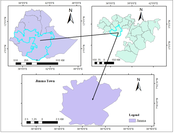
This study took place in the Jimma Zone of the Oromia National Regional State, a region renowned for its cultivation of cash crops like Buna. Situated in the northwestern part of Ethiopia, the study area can be found at 7.6670 latitude and 36.8330 longitude, a distance of 450 km from the capital city of Addis Ababa. With its unique location and rich agricultural heritage, the Jimma Zone is an ideal location for in-depth research and analysis.
The study employed the descriptive time-series analysis method and ARIMA model to forecast the annual and monthly temperature and rainfall of the study area. Both traditional Python-Jupyter Notebook and ARIMA model toolsets in MATLAB, using the Python-Jupyter Notebook platform, were utilized for this purpose. The results of seasonal time-series trends and annual analysis were subjected to descriptive statistics to filter out trends and seasonalities.
2.2.1. Temperature and Rainfall Time Series Analysis Method
In a study comparing the links between weather variables and hospitalizations for viral pneumonia, including influenza, during normal weather periods and El Niño events in three regions of California, time series analysis was employed. The study utilized temperature variables and precipitation, which were analyzed using time series analysis techniques. In theory, time series data should be stationary to enable accurate forecasting
[13]
Ebi, K. L. e. a., Association of normal weather periods and El Niño events with viral pneumonia hospitalizations in females, California 1983–1998. A. merican Journal of Public Health 91, 2001: p. 1200-1208.
[13]
. Stationarity refers to the covariance of the variable of interest not being dependent on time but rather on lag. Statistical time series methods and even modern machine learning methods benefit from the clearer signal in the data. When dealing with large input data volumes and greater precision is required, traditional time series methods may fail, and deep learning methods can be used to find the best model of unknown nonlinear relationships in time series data. Deep learning LSTM algorithms can be utilized to take advantage of the extra analytics power of mixed properties data, where both stationary and non-stationary features coexist, for better performance.
[14]
Khan, S. M., Application of Deep Learning LSTM and ARIMA Models in Time Series Forecasting: A Methods Case Study analyzing Canadian and Swedish Indoor Air Pollution Data.. Austin J Med Oncol., 2022. 9(1): p. 1073.
[14]
.
2.2.2. Augmented Adfuller Test
In 1976, Box and Jenkin from the University of Pennsylvania introduced the autoregressive integrated moving average (ARIMA) model for predicting stationary time series without seasonal variation
[15]
Box, P. E. G. and M. G. Jenkins, Times Series Analysis, Forecasting and Control; Taylor & Francis on behalf of the American Statistical Association (USA). San Francisco, CA, USA, (1976).
[15]
. The ARIMA model has three parameters: p, d, and q. the order of auto-regression is denoted by p, the order of differencing needed to make the time series stationary is represented by d, and q is the order of moving averages. Auto-regression is a technique that predicts a variable by comparing the recent pattern to its predecessors. On the other hand, a regression model employs errors from a previous forecast to predict the outcome of a subsequent forecast. Out of several unit root tests, Augmented Adfuller is one of the widely used tests. It uses an autoregressive model and optimizes an information criterion across different lag values
[16]
Manzoor, A. and A. Mansaf, An Intelligent IoT-Cloud-Based Air Pollution Forecasting Model Using Univariate Time-Series Analysis.. Arabian Journal for Science and Engineering., 2023.
[16]
. The null hypothesis (H0) of the test is that the time series can be represented by a unit root and that it is not stationary. The alternate hypothesis (H1) rejects the null hypothesis and suggests that the time series is stationary and does not have time-dependent structure. We interpret the result using the p-value from the test. A p-value below a threshold (10%, 5%, or 1%) indicates that we reject the null hypothesis (stationary). In contrast, a p-value above the threshold indicates that we fail to reject the null hypothesis (non-stationary). If the p-value is greater than 0.05, we fail to reject the null hypothesis (H0), meaning the data has a unit root and is non-stationary. However, if the p-value is less than or equal to 0.05, we reject the null hypothesis (H0), indicating that the data does not have a unit root and is stationary. The stats models library provides the fuller () function that implements the test. In the case of this study, the Adfuller test results showed that the p-value was less than 0.05, so the data is stationary. I ran this test for the study area datasets, and the results of the Adfuller test are presented in Table 1 below.
Table 1. Result of Adfuller Test.
Adfuller Test
Data
ADF Statistic
-31.58
p-value
0.047
#lag Used
0.047
number of observations used
96
Critial Values: 1%,
-3.512
Critial Values: 5%,
-2.897
Critial Values: 10%,
-2.586
The ADF test's null hypothesis is that the data is not stationary. In this study, the researchers evaluated the test statistics for the study area's data. They found that it was greater than the critical value (at 10%) and the p-value was less than the significant value of 0.05%. Therefore, they failed to reject the null hypothesis and considered the data as stationary. Consequently, the researchers made the data stationary by differencing and decomposing it. The correlation (C) and partial correlation (PC) are used to determine if the data is autoregressive or not. If C tails off gradually and cuts off after p lags, it's an AR(p) model. If C cuts off after q lags tails off gradually, the model is MA(q). Finally, if both C tails off gradually, the model should be ARIMA (p, q). In this study, the sample data showed that C tailed off gradually, which is why the AR model was used in the ARIMA model.
2.2.3. Seasonal ARIMA/SARIMA Model
In a SARIMA model, a non-seasonal ARIMA (p, d, q) is used in combination with seasonal components (P, D, Q) to represent several time steps that make up a period m. Seasonal AR, season moving average, and P, Q signify seasonal differencing, with D
[17]
Hecke, T. V., Time series analysis to forecast temperature change. University College Ghent, 2000.
[17]
. The acronym ARIMA stands for Auto-Regressive Integrated Moving Average. Algebraically, the ARIMA model can be defined by:
At time t = 1,..., n, where ǫt−j (j = 0, 1,..., q) are the lagged forecast errors. The p+q+1 unknown parameters μ, b1,... bp and a1,... aq are determined by minimizing the squared residuals. In the first part of the right-hand side of (1), the dependent variable is predicted based on its values at earlier periods. This is the autoregressive (AR) part of the equation (1). In the second part, the dependent variable y also depends on the values of the residuals at earlier periods, which may be regarded as prior random shocks. This is the moving average (MA) part of the equation. The researcher analyzing a given time series must find the relevant parameters of the ARIMA (p, d, q) model, where p is the number of autoregressive terms, d is the number of non-seasonal differences, and q is the number of lagged forecast errors in the prediction equation. Two goals must be met, namely to find the most effective model and to restrict the number of parameters. The residuals should also fulfill the conditions of independence and normality
[17]
Hecke, T. V., Time series analysis to forecast temperature change. University College Ghent, 2000.
[17]
.
As for time series prediction, historical data should be stationary where the covariance of the variable of importance is a function of lag, not of time. The datasets are non-stationary, as demonstrated by descriptive and inferential statistical Adfuller tests (Table 2), which indicate that both datasets had monthly trends and seasonal changes in temperature and rainfall (Figures 2-5). Stationary data with random fluctuations of radon levels is suitable for assigning to an ARIMA (Auto-Regressive Integrated Moving Average) model that predicts future trends (Figure 6).
3. Results and Discussions
3.1. Time Series Variation of Monthly and Annual Precipitation and Temperature
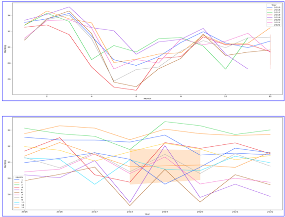
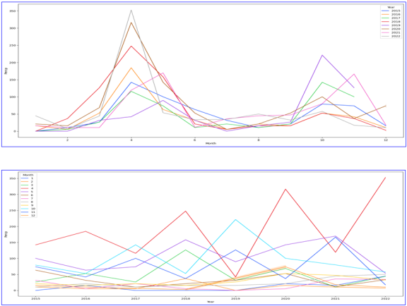
The graph presented in Figure 2 below illustrates the time series variation of precipitation for the study station. The results of the precipitation data reveal some interesting patterns. Firstly, it is observed that the maximum rainfall occurred from March to May for the years 2022, 2021, and 2020. This indicates that these months experienced the highest amount of rainfall during these years. Additionally, the precipitation data identified that the maximum rainfall was recorded for the years 2017, 2018, and 2019 during the months of October to November. This suggests that during these months, there was a significant amount of rainfall as compared to the rest of the year. Overall, the data highlights the seasonal variability of precipitation for the study station and provides useful insights into the rainfall patterns for the past few years. The study conducted a thorough analysis of the annual maximum precipitation data spanning from the years 2015 to 2022. The results of the analysis showed that the years 2020 and 2022 had the highest annual maximum precipitation, with precipitation peaks occurring specifically in the month of April. In contrast, the years 2019 and 2021 recorded the lowest maximum precipitation in April. Furthermore, it was found that the year 2019 experienced its highest precipitation in the month of October, while the year 2021 saw its highest precipitation in May. These findings provide a detailed understanding of the patterns of precipitation over the years, which can be valuable in various fields such as agriculture, hydrology, and environmental studies.
Figure 2. Monthly and annual precipitation variation over the years (2015–2022) at Jimma station.
3.2. Time Series Variation of Monthly and Annual Maximum Temperature
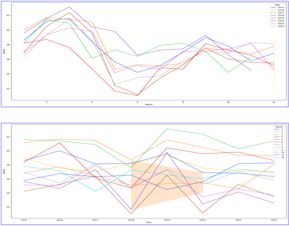
The graph displayed in figure 3 below illustrates the maximum temperature time series on a monthly and annual basis. The analysis of the maximum temperature data reveals that over the years, the highest temperatures were recorded in May, December, and November. However, starting from the year 2019, there has been a noticeable decline in the maximum temperature results recorded in December, while the maximum temperature results in April have been on an upward trend. Furthermore, the maximum temperature recorded in June and July during 2018 and 2019 showed unexpected results with a significant decrease.
The maximum temperature throughout the year was recorded in January, February, and March, while the annual maximum temperature in April, May, June, and July was comparatively lower than the other months. This was due to the onset of the spring season in Ethiopia, which brings the first rainfall of the year.
Figure 3. Monthly and annual Maximum Temperature variation over the years (2015–2022) at Jimma station.
3.3. Time Series Variation of Monthly and Annual Minimum Temperature
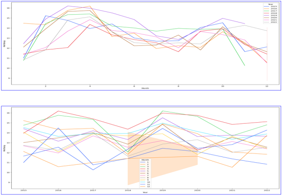
Figure 4 below presents a map of the time series for minimum temperatures on a monthly and annual basis. The minimum temperature for all years was recorded in December, November, and January. However, in 2016 and 2019, the minimum temperature results for December, November, and January have shown an increasing trend. Furthermore, the monthly minimum temperature recorded in April for all years was relatively higher than that of the other months.
Figure 4. Monthly and annual Minimum Temperature variation over the years (2015–2022).
Throughout the years, it has been observed that the minimum annual temperature tends to occur during the months of June, July, August, and September, while the maximum annual minimum temperature is typically recorded in January, February, March, and April. These results can be attributed to the fact that these months fall within the winter season in Ethiopia, during which the sun is situated in the northern hemisphere.
3.4. Time Series Variation of Monthly and Annual Average Temperature
The graph in Figure 5 below shows the monthly and annual average temperature time series. The highest average temperatures for all years were recorded in February and March. Additionally, in 2018 and 2020, the average temperature results decreased in June and July, while in 2017 and 2019, the average temperature increased during those months. In April, the monthly minimum temperature recorded was higher than in other months for all study years. Furthermore, between 2015 to 2017 and 2021 to 2022, the average temperatures for all months identified the maximum average temperature respectively.
Based on the findings of the annual temperature study conducted in 2016, 2021, and 2022, there was a sudden decrease in the average temperature during May, June, and July. On the other hand, the average temperature showed an increase during January, February, and March for all years under study.
Figure 5. Monthly and annual Average Temperature variation over the years (2015–2022) at Jimma station.
3.5. Correlation Between Precipitation and Average Temperature
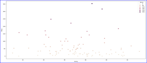
An analysis was conducted to determine the correlation between the average temperature and precipitation. This was done by creating a scatter plot diagram, which is presented in Figure 6. The highest correlation was found when the rainfall was less than 60mm and the average temperature ranged between 34°C to 39°C.
Figure 6. Correlation between precipitation and Annual Average Temperature variation over the years (2015–2022).
Table 2 below presents the correlation matrix that includes all the available data. As per the findings of this study, the correlation between precipitation and the average temperature is observed to be very low, with a value of -0.08806. This indicates that the correlation is either close to zero or in the negative territory. On the other hand, the maximum temperature and the average temperature exhibit the most significant correlation, with a value of 0.962518. This is followed by the correlation between minimum temperature and average temperature.
Table 2. Overall data correlation matrix. MaxTemp (Maximum Temperature), MinTemp (Minimum Temperatre), Averg (Average Temperature), and Percp (Percipitation).
Month
Year
MaxTemp
MinTemp
Averg
Percp
Month
1
0.014487
-0.36693
-0.25032
-0.40006
0.000884
Year
0.014487
1
-0.1021
-0.05973
-0.10856
0.113805
MaxTemp
-0.36693
-0.1021
1
0.22302
0.962518
-0.20703
MinTemp
-0.25032
-0.05973
0.22302
1
0.479047
0.353547
Averg
-0.40006
-0.10856
0.962518
0.479047
1
-0.08806
Percp
0.000884
0.113805
-0.20703
0.353547
-0.08806
1
4. Conclusion
The two most critical climatic variables for analyzing climate patterns are the mean monthly temperature and total monthly precipitation, which can be easily obtained from weather station records
[4]
Mulomba, P. M. and C. González-García, Time Series Analysis of Climatic Variables in Peninsular Spain. Trends and Forecasting Models for Data between 20th and 21st Centuries. Climate, 2021. 9(119).
[4]
. For this study, temperature and precipitation data were collected from the Global Historical Climatology Network-Monthly (GHCN-M) dataset provided by the National Centers for Environmental Information (NCEI) during the study periods from 2015 to 2022. The Python 3.1.1 on Anaconda Jupyter Notebook and the matplotlib 3.2.1 package for data visualization were used for monthly and annual temperature and precipitation time series analysis. The results indicate that the maximum rainfall occurred between March and May for 2020, 2021, and 2022, while for 2017, 2018, and 2019, the maximum rainfall was recorded in October, December, and November. The annual maximum rainfall occurred in 2020 and 2022. The annual maximum temperature for all years was recorded in January, February, and March, while the annual minimum temperature was recorded in June, July, August, and September. Additionally, the annual average temperatures occurred in January, February, and March. The analysis of temperature and rainfall time series is essential for monitoring climate change and sustainable development, providing valuable insights into temperature and rainfall trends for governmental and private sectors working on climate change. The researcher suggests that this paper or data can be used by others to study the prediction of temperature and rainfall using different climate models.
Abbreviations
GHCN-M
Global Historical Climatology Network – Monthly
NCEI
National Centers for Environmental Information
TS
Time Series
RS
Remote Sensing
EO
Earth Observation
LiDAR
Light Detection and Ranging
GAM
Generalized Additive Models
GEE
Generalized Estimating Equation
ARIMA
Autoregressive Intergrated Moving Average
PC
Partial Correlation
Author Information
Unit of Geodesy, Geomatics’ and Gravimetry; Institute of Geophysics, Space Science and Astronomy; Addis Ababa University, Addis Ababa, Ethiopia
Ethical Consideration
The research didn’t involve human subject due that it is not applicable.
Consent for Publication
I have agree to submit journal of climate change and approved the manuscript for submission.
Author Contributions
Wendafiraw Abdisa Gemmechis is the sole author. The author read and approved the final manuscript.
Funding
No funding information.
Data Availability Statement
The data is included in the manuscript.
Conflicts of Interest
The author declares no conflicts of interest.
References
[1]
McMichael, A. J., et al., eds. Climate change and human health Risks and Responses. World Health Organization Geneva. 2003.
[2]
Belay, F. E., et al., Spatio-Temporal Variability and Time Series Trends of Monthly and Seasonal Rainfall Over Northwestern Ethiopia.. Global Journal of Environmental Research, 2020. 14(2): p. 45-54.
[3]
Ye L. M., G. X., et al., Time-series modeling and prediction of global monthly absolute temperature for environmental decision making.. Adv. Atmos. Sci.,, 2013. 30(2): p. 382-396.
[4]
Mulomba, P. M. and C. González-García, Time Series Analysis of Climatic Variables in Peninsular Spain. Trends and Forecasting Models for Data between 20th and 21st Centuries. Climate, 2021. 9(119).
[5]
Markéta, P., et al., E-TRAINEE: OPEN E-LEARNING COURSE ON TIME SERIES ANALYSIS IN REMOTE SENSING. The International Archives of the Photogrammetry, Remote Sensing and Spatial Information Sciences,, 2023. XLVIII-1/W2-2023.
[6]
Waqas, M., et al., Potential of Artificial Intelligence-Based Techniques forRainfall Forecasting in Thailand. A Comprehensive Review. Water 2023. 15(2979).
[7]
Jones, P. D. and A. Moberg, 2003: Hemispheric and large-scale surface air temperature variations:. An extensive revision and an update to 2001. Climate, 2001. 16: p. 206-223.
[8]
Hansen, J. M., et al., Global temperature change.. Proc. National Academy of Sciences USA,, 2006. 103: p. 14288-14293.
[9]
Rahmstorf, A. S., et al., Recent climate observations compared to projections.. Science,, 2007. 316.
[10]
IPCC, Detection of climate change and attribution of causes. in Climate Change 2001: The Scientific Basis. Contribution of Working Group I to the Third Assessment Report of the Intergovernmental Panel on Climate Change, J. T. Houghton et al., Eds., Cambridge University Press. 2001. p. 44.
[11]
Lee, H. J. and K.-T. Sohn, Prediction of monthly mean surface air temperature in a region of China.. Adv. Atmos. Sci.,, 2007. 24: p. 503-508.
[12]
Murat, M., et al., Forecasting Daily Meteorological Time Series Using ARIMA and Regression Models. Int. Agrophys., 2018. 32.
[13]
Ebi, K. L. e. a., Association of normal weather periods and El Niño events with viral pneumonia hospitalizations in females, California 1983–1998. A. merican Journal of Public Health 91, 2001: p. 1200-1208.
[14]
Khan, S. M., Application of Deep Learning LSTM and ARIMA Models in Time Series Forecasting: A Methods Case Study analyzing Canadian and Swedish Indoor Air Pollution Data.. Austin J Med Oncol., 2022. 9(1): p. 1073.
[15]
Box, P. E. G. and M. G. Jenkins, Times Series Analysis, Forecasting and Control; Taylor & Francis on behalf of the American Statistical Association (USA). San Francisco, CA, USA, (1976).
[16]
Manzoor, A. and A. Mansaf, An Intelligent IoT-Cloud-Based Air Pollution Forecasting Model Using Univariate Time-Series Analysis.. Arabian Journal for Science and Engineering., 2023.
[17]
Hecke, T. V., Time series analysis to forecast temperature change. University College Ghent, 2000.
Gemmechis, W. A. (2024). Climate Change Trend Using Descriptive Time Series Technique in Machine Learning: A Case of Jimma Zone, Southwestern Ethiopia. International Journal of Environmental Monitoring and Analysis, 12(3), 48-57. https://doi.org/10.11648/j.ijema.20241203.12
Gemmechis, W. A. Climate Change Trend Using Descriptive Time Series Technique in Machine Learning: A Case of Jimma Zone, Southwestern Ethiopia. Int. J. Environ. Monit. Anal.2024, 12(3), 48-57. doi: 10.11648/j.ijema.20241203.12
Gemmechis WA. Climate Change Trend Using Descriptive Time Series Technique in Machine Learning: A Case of Jimma Zone, Southwestern Ethiopia. Int J Environ Monit Anal. 2024;12(3):48-57. doi: 10.11648/j.ijema.20241203.12
@article{10.11648/j.ijema.20241203.12,
  author = {Wendafiraw Abdisa Gemmechis},
  title = {Climate Change Trend Using Descriptive Time Series Technique in Machine Learning: A Case of Jimma Zone, Southwestern Ethiopia
},
  journal = {International Journal of Environmental Monitoring and Analysis},
  volume = {12},
  number = {3},
  pages = {48-57},
  doi = {10.11648/j.ijema.20241203.12},
  url = {https://doi.org/10.11648/j.ijema.20241203.12},
  eprint = {https://article.sciencepublishinggroup.com/pdf/10.11648.j.ijema.20241203.12},
  abstract = {Understanding climate variability and monitoring time-series trends of temperature and rainfall is crucial for the sustainable development of our planet. This study utilized historical data from the Global Historical Climatology Network-Monthly (GHCN-M) provided by the National Centers for Environmental Information (NCEI) to analyze the temperature and rainfall data from 2015 to 2022. The analysis was conducted using Python 3.1.1 on Anaconda Jupyter Notebook and the package matplotlib 3.2.1 was used for data visualization. The results revealed a pattern of maximum rainfall between March to May for the years 2020, 2021, and 2022, while for the years 2017, 2018, and 2019, the maximum rainfall was recorded in October, December, and November. Additionally, the annual maximum rainfalls were recorded in the years 2020 and 2022, and the annual maximum temperatures for all study years were recorded in January, February, and March months. On the other hand, the annual minimum temperatures for all study years occurred in June, July, August, and September months. Similarly, annual average temperatures were recorded in January, February, and March months. This study emphasizes the importance of monitoring climate change and its impacts on our planet. By understanding climate variability and time-series trends, we can better prepare for the future and work towards a sustainable world.
},
 year = {2024}
}
TY  - JOUR
T1  - Climate Change Trend Using Descriptive Time Series Technique in Machine Learning: A Case of Jimma Zone, Southwestern Ethiopia

AU  - Wendafiraw Abdisa Gemmechis
Y1  - 2024/07/02
PY  - 2024
N1  - https://doi.org/10.11648/j.ijema.20241203.12
DO  - 10.11648/j.ijema.20241203.12
T2  - International Journal of Environmental Monitoring and Analysis
JF  - International Journal of Environmental Monitoring and Analysis
JO  - International Journal of Environmental Monitoring and Analysis
SP  - 48
EP  - 57
PB  - Science Publishing Group
SN  - 2328-7667
UR  - https://doi.org/10.11648/j.ijema.20241203.12
AB  - Understanding climate variability and monitoring time-series trends of temperature and rainfall is crucial for the sustainable development of our planet. This study utilized historical data from the Global Historical Climatology Network-Monthly (GHCN-M) provided by the National Centers for Environmental Information (NCEI) to analyze the temperature and rainfall data from 2015 to 2022. The analysis was conducted using Python 3.1.1 on Anaconda Jupyter Notebook and the package matplotlib 3.2.1 was used for data visualization. The results revealed a pattern of maximum rainfall between March to May for the years 2020, 2021, and 2022, while for the years 2017, 2018, and 2019, the maximum rainfall was recorded in October, December, and November. Additionally, the annual maximum rainfalls were recorded in the years 2020 and 2022, and the annual maximum temperatures for all study years were recorded in January, February, and March months. On the other hand, the annual minimum temperatures for all study years occurred in June, July, August, and September months. Similarly, annual average temperatures were recorded in January, February, and March months. This study emphasizes the importance of monitoring climate change and its impacts on our planet. By understanding climate variability and time-series trends, we can better prepare for the future and work towards a sustainable world.

VL  - 12
IS  - 3
ER  -