Biodiversity and the Community Structure of Chromista Cavalier-Smith, 1981 in Nyong and Kienke River Mouths (South-Cameroon)

Christelle Chimene Mokam; Andrea Sarah Kenne Toukem; Christian Dongmo Teufack; Fabien Tresor Amougou Dzou; Sedrick Junior Tsekane; Mohammadou Moukhtar; Auguste Pharaon Mbianda; Martin Kenne

doi:doi:10.11648/j.ijee.20240901.12

Research Article |

| Peer-Reviewed

Biodiversity and the Community Structure of Chromista Cavalier-Smith, 1981 in Nyong and Kienke River Mouths (South-Cameroon)

Christelle Chimene Mokam

, Andrea Sarah Kenne Toukem

, Christian Dongmo Teufack

, Fabien Tresor Amougou Dzou

, Sedrick Junior Tsekane

, Mohammadou Moukhtar

, Auguste Pharaon Mbianda

, Martin Kenne^*

Published in International Journal of Ecotoxicology and Ecobiology (Volume 9, Issue 1)

Received: 1 March 2024 Accepted: 18 March 2024 Published: 2 April 2024

Views: Downloads:

Download PDF

Share This Article

Twitter
Linked In
Facebook

Abstract

A survey was undertaken from March to June 2014 on the biodiversity and the community structure of Chromista Cavalier-Smith, 1981 in Nyong and Kienke River mouths (South-Cameroon). In each river, raw waters were collected from upstream to downstream at four sites. Cells were counted using the Malassez cells procedure and species were identified. A total of 10427.1x10⁵ cells corresponded to three phyla, eight classes, 23 orders, 32 genera and 40 species (24 freshwater species (60.0% of total species richness and total collection respectively), three marine species (7.5% and 2.4% of the total species richness; and total collection respectively), and one brackish water specialist in Kienke (2.5% and 5.1%), 13 tolerant species (32.5% and 32.6%)). The trophic diatom index revealed undisturbed conditions with no or little alteration of human origin and a low organic pollution (oligotrophic or mesotrophic state) (Nyong: TDI=52.7; Kienke: TDI=69.7; pooled assemblage: TDI=65.0). A low species richness was detected (richness ratio in Nyong: d=0.008; Kienke: d=0.003; pooled rivers: d=0.004), a high species diversity (Shannon index close to maximum) (Nyong: H’=2.742 and H’_max=2.996; Kienke: H’=2.685 and H’_max=2.996; pooled rivers: H’=3.245 and H’_max=3.689), a very low dominance by a few species (Berger-Parker index close to 0) (Nyong: I_BP=0.156; Kienke: I_BP=0.175; pooled rivers: I_BP=0.134), and Hill’s ratio were close to 1 (Nyong: Hill=0.819; Kienke: Hill=0.803; pooled rivers: Hill=0.722). The community was highly even with a high value of the Pielou’s evenness close to 1 (Nyong: J=0.915; Kienke: J=0.896; pooled rivers: J=0.880). Two useful species and one harmful species to fish were rare in Kienke. Species exhibited in Kienke and pooled data in rainy season, a positive global net association while it was negative in Nyong. Assemblage fitted Preston’s model in Nyong with a high environmental constant in the dry season (m’=1.469), low constant in the rainy season (m’=0.947) and the pooled seasons (m’=0.853). In Kienke constants were low (dry season: m’=0.574; rainy season: m’=0.566; pooled seasons: m’=0.581) suggesting a evolved community in less disturbed environments where the majority of species showed moderate abundances. In the dry season, the pooled assemblage functionned on the basis of maintaining a complex information network (close to ecological balance) developed at spatio-temporal scales (ZM model) and it presented a low force of regeneration (fractal dimension of the distribution of individuals among species (1/γ)=0.925<1). The evolved oligotrophic state (close to natural balance) of the chromists’ community should be preserved and protected and the studied rivers classified as reference.

Published in	International Journal of Ecotoxicology and Ecobiology (Volume 9, Issue 1)
DOI	10.11648/j.ijee.20240901.12
Page(s)	28-55
Creative Commons	This is an Open Access article, distributed under the terms of the Creative Commons Attribution 4.0 International License (http://creativecommons.org/licenses/by/4.0/), which permits unrestricted use, distribution and reproduction in any medium or format, provided the original work is properly cited.
Copyright	Copyright © The Author(s), 2024. Published by Science Publishing Group

Keywords

Freshwater Species, Microalgae, Species Composition, Useful Species, Assemblage Functioning, Water Quality

1. Introduction

According to the AlgaeBase, 50,589 species of living algae and 10,556 fossil species are documented, referred to four kingdoms (Eubacteria Woese & Fox, 1977; Chromista Cavalier-Smith, 1981; Plantae Haeckel, 1866; and Protozoa Goldfuss, 1818), 14 phyla, and 63 classes

[1]

. Algae are the third most speciose grouping of plant-like after the flowering plants (≈382,000 species) and fungi (≈170,000 species, including lichens)

[1]

. The most species-rich phylum is the golden and brown algae Heterokontophyta Moestrup, 1992 with 18 classes and 21,052 living species dominated by the diatoms class Bacillariophyceae Dangeard, 1933 with 18,673 species (16,427 living species and 2,239 fossil)

[1]

. The next most species-rich phyla are the red algae Rhodophyta Wettst., 1901 (7,276 living species), the oxygenic photosynthetic green algae (6,851 living species), the blue-green algae (Cyanobacteria Stanier, 1973 or Cyanobacteriota Oren et al. 2022: 5,723 living species), the charophytes (4,950 living species, including Charophyceae with 511 living species, and Zygnematophyceae with 4,335 living species), Dinoflagellata (2956 living species, including Dinophyceae, 2,828 species), and haptophytes (Haptophyta: 1,722 species with 517 living species)

[1]

. Chromista is distinguished from Plantae and other phytoplankton because of its more complex chloroplast-associated membrane topology and rigid tubular multipartite ciliary’s hairs

[2]

. Chromista (colored algae) possess a brown plastid resulting from a primary or secondary endosymbiosis with red algae

[3]

. They represent one of the five eukaryotic kingdoms in the seven-kingdom classification of life

[3-9]

. Nowadays Chromista comprises six divisions [golden or golden-brown algae Chrysophyta Pascher (1914); red algae Cryptophycophyta; Haptophyta Caval.-Sm., 1986 \l "cite_note-AlgaeBASE15_août_2017-1"; brown algae Phaeophyta Kjellman, 1891; dinoflagellates Pyrrophycophyta; and yellow-green algae Xanthophyta Allorge, 1930, emend. Fritsch, 1935]. It compreses seven classes, 53 orders, 151 families, 487 genera, 2,029 species, one subspecies and 138 varieties

[10]

. Chysophyta includes one class ( Chrysophyceae Pascher, 1914), 10 orders, 23 families, 74 genera, 288 species, and 36 varieties

[10]

. Cryptophycophyta includes one class, six families, 14 genera, 83 species, and four varieties

[10]

. Haptophyta includes one class, three orders, 10 families, 45 genera, and 90 species

[10]

. Phaeophyta includes one class, 12 orders, 35 families, 156 genera, 498 species, and 51 varieties

[10]

. Pyrrophycophyta includes two classes, 20 orders 57 families, 145 genera, 913 species, one subspecies, and 39 varieties

[10]

. Xanthophyta includes about 600 species and many of the 100 known genera contain only a few species

[6]

. It includes one class (Xanthophyceae), seven orders, 20 families 53 genera 157 species, and eight varieties,

[10]

. Based on the number of families, the descending ranking of the well-represented classes is as follows: the diatoms Bacillariophyceae (92 families; 3,399 species), Dinophyceae (55 families; 911 species), Phaeophyceae (35 families; 498 species), Chrysophyceae (23 families; 288 species), Xanthophyceae (20 families; 157 species), Prymnesiophyceae (10 families; 90 species), Cryptophyceae (six families; 83 species), Chloromonadophyceae (two families; two species), and Cyanophyceae (more than 150 genera; 7,500 species). But these numbers are clearly below reality because the group has remained unknown to scientists for a long time and several forms are undetermined

[7]

. Chromists (colored algae) include the majority of marine species, brackish water specialists, freshwater species and terrestrial species as well as heterotrophic protists whether marine, brackish or freshwater. For these reasons, the Chromista kingdom is very important for the ocean and freshwater ecology

[11]

. As photosynthetic species they are essential primary producers of the aquatic food webs for fish and other macro invertebrates as well as mocrovertebrates, and they also have an economic importance as oxygen producers

[12]

, or as bioindicators of the water quality (due to the preference of each species for aquatic environments with very specific physicochemical characteristics)

[13]	Zalat, A. A., Nitychoruk, J., Chodyka, M., Pidek, I. A., Welc, F. Recent and fossil freshwater diatoms of Poland: taxonomy, distribution and their significance in the environmental reconstruction. Part 1. Coscinodiscophyceae, Mediophyceae and Fragilariophycidae. John Paul II University of Applied Sciences, Biała Podlaska; 2022, pp. 1-306
[14]	Jahn, R., Kusber, W. H., Romero, O. E. Cocconeis pediculus Ehrenberg and C. placentula Ehrenberg var. placentula (Bacillariophyta): Typification and taxonomy. Fottea. 2009, 9(2), 275–288. https://doi.org/10.5507/fot.2009.027 View Article
[15]	Hecky, R. E., Kilhan, P. Diatoms in Alkaline, Saline Lakes: Ecology and Geochemical Implications. Limnology and Oceanography. 1973, 18(1), 53-71. https://doi.org/10.4319/LO.1973.18.1.0053 View Article
[16]	Spaulding, S. A., Potapova, M. G., Bishop, I. W., Lee, S. S., Gasperak, T. S., Jovanovska, E., Edlund, M. B.. Diatoms.org: supporting taxonomists, connecting communities. Diatom Research. 2021, 36(4): 291-304. https://doi.org/10.1080/0269249X.2021.2006790 View Article
[17]	Houk, V.; Klee, R., Tanaka, H. Atlas of freshwater centric diatoms with a brief key and descriptions, Part III, Stephanodiscaceae A, Cyclotella, Tertiarius, Discostella. Fottea. 2010, 10(Supplement), 1–498.
[18]	Krammer, K., Lange-Bertalot, H. Bacillariophyceae, 2nd part: Bacillariaceae, Epithemiaceae, Surirellaceae. In Süsswasserflora von Mitteleuropa, Band 2/2. Ettl, H., Gerloff, J., Heynıg, H., Mollenhauer, D., Eds., Gustav Fischer Verlag, Stuttgart, Germany; 1988, pp. 1-596.
[19]	Krammer, K, Lange-Bertalot, H. Bacillariophyceae, 3. Teil: Centrales, Fragilariaceae, Eunotiaceae. In Süsswasserflora Von Mitteleuropa, Band 2/3. Ettl, H., Gerloff, J., Heynıg, H., Mollenhauer, D., Eds., Gustav Fischer Verlag, Stuttgart, Germany; 1991, pp. 1-596.
[20]	Mohanty, T. R.,•Tiwari, N. K.,•Kumari, S.,•Ray, A.,•Manna, R. K., Bayen, S.,•Roy, S.,•Gupta, S. D.,•Ramteke, M. H.,•Swain, H. S., Bhor, M.,•Das, B. K. Variation of Aulacoseira granulata as an eco pollution indicator in subtropical large river Ganga in India: a multivariate analytical approach. Environmental science and pollution research international. 2022, 29(25), 37498-37512 https://doi.org/10.1007/s11356-021-18096-9 View Article
[21]	Taylor, J. C., Harding, W. R., Archibald, C. G. M. An Illustrated Guide to Some Common Diatom Species from South Africa. WRC Report TT 282/07. Water Research Commission. Gezina, Pretoria, South Africa; 2007, pp. 1-225.
[22]	DeColibus, D. “Tabellaria flocculosa (Roth) Kütz. 1844. In Diatoms of North America”. Available from https://diatoms.org [Accessed 01 March 2024]. View Article

[13-22]

, or as biofertilizer from their N-fixing endosymbionts [for example similar to other species of Epithemia, Ep. turgida (Baccillariophyceae: Rhopalodiales: Rhopalodiaceae) contains N-fixing Cyanobacteria, these endosymbionts enable algae cells to become abundant in microhabitats with a low N/P ratio and they are frequently abundant as epiphyte on Cladophora and other coarse filamentous algae (particularly in western rivers)

[23]

, or as detoxifiers of wastewater polluted with antibiotics (case of Chaetoceros muelleri (Bacillariophyta: Baccillariophyceae: Chaetocerotanae incertae sedis: Chaetocerotaceae) which is an appealing solution to remove certain antibiotics such as sulfamethoxazole and ofloxacin from wastewater)

[24]

. Several species of Chromista show a detrimental ecological impact as producers of toxins harmful to aquatic living organisms

[25-30]

. This is the case of the genus Ceratium (Dinophyceae: Gonyaulacales: Ceratiaceae) which sometimes causes dramatic blooms in lakes and responsible of fish mortality

[31]

. This is also the case of the genus Chaetoceros which is non-toxic to humans but harmful to fish and invertebrates (especially in intensive aquaculture systems) by damaging or clogging their gills

[32]

. Several species of Chromista are responsible of zoonoses, as the case of oomycetes Saprolegnia responsible of the saprolegnosis pathology in fish

[33]

and the case of labyrinthulomycetes that cause diseases in aquatic animals

[34]

. Apart from the harmful impact reported in several species, some species (case of labyrinthulomycetes) live as commensals or mutualists within the guts and tissues of aquatic invertebrates and they are saprobic on animal faeces and molluscs shells

[34]

. These potentialities make Chromists good bio-indicators of the water quality of life.

Nyong and Kienke river mouths (South Cameroon) are source of drinking water and fishing activities

[35]

. Residents depend on artisanal small-scaled fishing using canoes for household consumption

[36, 37]

and to supply the neighbouring urban areas

[37]

. Nevertheless, the demand is growing and fishermen complain about the deterioration of the fish resources for many reasons including irresponsible fishing practices (use of pesticides) and the poor land use management

[35]

. In this region, the community structure of aquatic micro algae is little known, except works concerning the tidal variation impact on the abundance of phytoplankton in the Nyong estuary

[38]

, seasonal variation of the water quality and the composition of the phytoplankton communities in lower Nyong estuary

[39]

, influence of physico-chemical parameters on the zooplankton dynamics in Kienke estuary

[40]

, the water quality, the biodiversity and abundance of blue-green algae in Nyong and Kienke River mouths

[41]

. But nothing is known concerning the zoonotic chromists, the toxigenic species, those useful for the nutrition of fish. The place occupied by harmful species in the community. The present study aimed to establish a baseline of information on the distribution of chromists, as a first step in evaluating the status and the occurrence of species known as bio-indicators of the aquatic life quality (useful species or producers of toxins).

2. Materials and Methods

2.1. Study Sites

Studies took place in 2014 at the Nyong river mouth mouth (03°16'40.71"N, 09°53'27.21"E and 03°14'58.41"N, 09°56'41.07"E) (Figure 1A) and the Kienke river mouth (02°22'4.06"N, 09°48'32.20"E and 02°17'56.31"N, 09°50'55.94"E) (Figure 1B), situated in the Southern coastal zone of Cameroon

[41]

. They are separated by a distance of 111.1 km. The prevailing climate is tropical with rainfall even during the driest months (December and January: 54.2 mm and 33.8 mm respectively)

[41, 42]

. The average air temperature ranges from 24.4°C (August) to 26.7°C (March) and the average rain fall ranges from 116 mm (January) to 340 mm (September). The average air humidity ranges from 84.0% (January to March) to 87.0% (September and October)

[41, 42]

. Four seasons are defined: a long dry season (late November-February), a short rainy season (March-June), a short dry season (July-August) and a long rainy season (early September-early November)

[36, 41]

. Soils are acidic, yellow ferralitic types, poor in minerals and organic matters and soils on gneiss outcrop cover the bulk between Campo and Kribi

[36, 41]

. Many streams crossing the region are influenced by the equatorial climate

[36, 41]

. The main rivers (Nyong, Lokoundje, Kienke, Lobe and Ntem) flow into the Atlantic Ocean and the watercourses are used by the residents for traditional fishing or as waterways using canoes or other navigation fleet

[36, 41]

. According to our recently published report

[41]

Nyong and Kienke river mouths belong to the warm category (temperature varying: 26.0 to 32.0°C). The pH varies from slightly acidic (pH=6.1) to slightly basic (pH=8.9). The transparency varies from 43.0 cm to 325 cm. The dissolved oxygen (DO) varies from 0.4 to 39.5 mg.l^-1. The five-day biochemical oxygen demand (BOD₅) varies from 5.0 to 50.0 mg.l^-1. The conductivity varies from 16.4 to 40,600.0 µS.cm^-1. The nitrite NO₂^- contents varies from 0 to 27.0 mg.l^-1. The nitrate NO₃^- contents varies from 0 to 9.9 mg.l^-1. Ammoniacal nitrogen (NH₄⁺) varies from 0.2 to 14.1 mg.l^-1. Orthophosphate (PO₄^3-) content varies from 0 to 2.0 mg.l^-1. The chlorophyll a content varies from 0.02 to 0.40 µg.l^-1. The biomass varies from 0.3 to 12.0 mg.c.l^-1. The faecal colliforms content varies from 75.0 to 1440.0 CFU. (100 ml)^-1 and the total suspended solids (TSS) varies from 0 to 33.3 mg.l^-1.

2.2. Sampling Design

Samplings were set up from March to June 2014 in the lower course of Nyong and Kienke mouths (Figure 1A), at the same sampling points presented in our recent publication

[41]

: four sites were selected 300 m from the shore of Nyong and 30 m from the shore for Kienke.

Download: Download full-size image

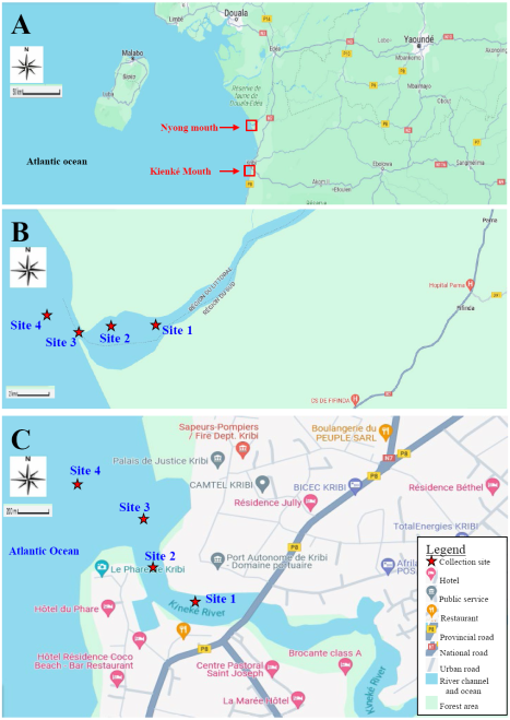
Figure 1. Location of the study sites in Southern coastal zone of Cameroon (southern province, Ocean department). A: Location of the Nyong and Kienke River mouths; B: Location of the collection sites in the Nyong River mouth; C: Location of the collection sites in the Kienke River mouth.

In each river, sampling sites were accessed using a wooden canoe (Nyong River mouth: site 1 at the beginning of the estuary (3°16'1.79"N, 9°56'25.72"E), site 2 at the middle of the estuary: (3°15'57.58"N, 9°55'31.13"E; 1.71 km from site 1), site 3 at the transition with ocean water (3°15'38.99"N, 9°54'16.28"E; 4.11 km and 2.47 km from site 1 and site 2 respectively) and site 4 located in the coastal area of the ocean (3°16'3.85"N, 9°53'45.64"E; 5.15 km, 3.4 km and 1.3 km from site 1, site 2 and site 3 respectively)) (Figure 1B)

[41]

. In the Kienke River mouth, locations of the sampling sites were: site 1 near a residential camp (2°19'20.40"N, 9°50'17.78"E), site 2 near a marshy area (2°20'14.06"N, 9°50'1.07"E; 1.9 km from site 1), site 3 at the transition with the ocean (2°20'55.01"N, 9°49'22.47"E; 1.8 km and 3.5 km from site 2 and site 1 respectively) and site 4 located in the coastal area of the ocean (2°21'17.29"N, 9°48'57.40"E; 4.8 km, 2.8 km and 1.1 km from site 1, site 2 and site 3 respectively) (Figure 1C)

[41]

. In each river mouth, as site 4 was situated far from the coast, an outboard boat permitted us to reach it. Samsung 14.2 Mega Pixels and Kodak 9.2 Mega Pixels cameras were used for the field shots. Coordinates of the sites were taken using a Garmin GPS. As presented in our recent publication

[41]

, three sampling sessions were done at each site (one in March, June and August respectively). The floating macro-particles were sampled and preserved in a water sample in plastic petri dishes hermetically closed with a plastic lid. For the microalgae detection, raw water was sampled at the water surface and one-meter depth using a Teflon ball and a two-litter Niskin messenger bottles and 150 ml transparent plastic polyethylene bottles and transported to the laboratory using a 100 ml Coleman cooler containing pieces of ice for temperature maintenance. Biological parameters of the sampled water (Chromista composition, identification and counting) were carried out at the micro algae laboratory of the Specialized Center for Research on Marine Ecosystems at Kribi (AquaSol service). Chromista cells concentration was determined using the Malassez cells. In case of insufficient homogeneity, the assembly was resumed using a new Malassez cell and the rehomogenized raw water. Chromista cells were identified and for each species, we counted the number of cells in ten randomly selected squared grid areas and the average number (n_i) of 10 Malassez’s squared grids and the final concentration were recorded as c_i=n_ix10⁵ cells.ml^-1. The total number of cells in volume “v” was estimated as n_i=c_iv and data were compiled in a species matrix database.

2.3. Species Identification and Data Analysis

Species identification was made using a Zeiss NR183268 series microscope and by referring to the descriptions, drawings, dimensions and photographs in available dichotomous keys

[43-46]

, Update name of species and their natural environment were obtained by referring to catalogs and websites available online

[11, 47-52]

. In each assemblage the weighed mean sensitivity (WWS) of the diatom community was determined and the trophic diatom index (TDI) was calculated. Data are given in terms of absolute and relative frequencies. Two independents percentages were compared using the Fisher’s exact test. For the simultaneous comparison of several percentages, the asymptotic p-value or the exact p-value was determined using the independent chi-square test or the Fisher-Freeman-Halton test from StatXact software version 3.1.

Alpha diversity analysis allowed the determination of 15 indexes using PAST 3.05 software: absolute abundance of the i^th species n_i, observed sample size n, relative abundance of the ith species p_i=(n_i/n)*100, species richness S, maximum abundance n₁ or n_max, Margalef’s index Mg=(S-1)/ln(n), richness ratio d=S/n (0 for the low-rich communities and +1 for the optimal species-rich communities), Shannon-Weaver diversity index H’ (0 for a single-species community and H’_max=ln(S) for the perfect species regularity of abundances), Simpson diversity index D (0 for a high diversities and +1 for a low diversities), Hill's N₁ diversity number (N₁=e^H’) for the estimated number of abundant species, Hill's N₂ diversity number (N₂=1/D) for the estimated number of co-dominants, Hill’s ratio N₂/N₁ with 0≤Hill≤+1, Pielou’s evenness index J=H’/ln(S) with 0 for a perfect heterogeneity of the assemblage and +1 for a perfect balance of abundances, and Berger-parker dominance index n_max/n with a low value reflecting a high diversity. Comparison of the species richness was performed using the individual rarefaction procedure. The non-parametric estimator Chao1 was used to estimate the theoretical species richness T and the sampling effort was estimated as (S/T)*100. The rank abundance plottings were used to illustrate the shape of the species abundance distributions (SADs). The goodness of fit of each SAD to a theoretical model was assessed by calculating the Pearson correlation between the logarithms of the numbers and the ranks of the species and interpreted as follows: r<-0.95 for a fit of a poor quality; r≈-0.95 for a approximative fit; r≈-0.98 for a satisfactory fit; and r≥-0.99 for an excellent fit. We used five commonly used theoretical models to fit the curves: broken-stick (BS), log-linear (LL) model, lognormal (LN) model, Zipf (Z) and Zipf-Mandelbrot (ZM). The best model was selected using the Akaike Information Criteria (AIC) or the Bayesian Information Criteria (BIC) (the best model presented the lowest AIC or BIC). The estimated sample size n* was adjusted to the observed size n using the correction factor n/n* and the corrected models were given. The package vegan of R 3.4.1 software helped us to adjust the SADs. BS model (McArthur’s model) or model of contiguous non-overlapping niches is based on a hypothetical form of sharing of biotope resources between the species present and in practical, this model is suitable for the analysis of communities in which inter-species relationships are elementary, competition being essentially limited to the level of the resource, such as physical space. This model has a single parameter x which represents the average abundance of species

[53]

. LL model (preemption model) suggests that numbers of species are distributed according to the geometrical progression (Motomura’s law) and the parameter m (Motomura’s environmental constant with 0≤m≤1) is the antilogarithm of the linear slope obtained by plotting species ranks (from the most to the least abundant) on the x-axis and the logarithms of corresponding abundances on the y-axis.

The species of the i^th rank in the ranking by decreasing abundance has therefore a number of individuals proportional to (k)(1-k)^(i-1), its logarithm being of the form (i−1)Log(1−k)+Log(k) which is a straight line of slope Log(1-k). This model depends on the maximum abundance of the top-ranking species n₁ and the Motomura’s environmental constant m (the rate of decrease in abundance by rank)

[54]

. According to the LN model, the logarithms of the abundances are distributed symmetrically and randomly, on either side of their mean, with a standard deviation of the logarithm distribution σ=square root of 1/m’, with m’ as the Preston’s environmental constant. The adjustment line Log(n_i)=f(P_i) with P_i the probit of the cumulative percentage linked to the ranks i, represents all the points, and makes it possible to calculate the theoretical abundances which would be those of n species if the nomocenosis was rigorously log-normal. For a species of rank i, we calculated the cumulative percentage linked to this rank k_i=100(i+0.5)/(S+1) when S was odd or k_i=100((i+1)+0.5)/(S+1) when S was even, and then the probit P_i=P_(ki) was determined. The package “ecotoxycology” of R 4.1.0 software helped us to determine the probits. The regression line between Log(n_i) and P_i has the relation: Log(n_i)=aP_i+b or n_i=(10^b)(10^a)^Pi where a and b represented the slope and the elevation respectively of the regression line Log(n_i)=f(P_i). Z model is based on the Zipf's law

[55]

, with abundances listed in descending order. Z model is defined from two statistics: Q which is the sum of all recorded abundances, also called sample size or the scale parameter (normalization constant) and γ (gamma) which is the decay coefficient or the average probability of appearance of a species and the relation is n_i=Q(i)^-γ where i represents the rank of the species ranked in decreasing order

[56, 57]

. ZM model n_i=Q(i+β)^-γ is a generalized model in which a new parameter β (beta) is added (the degree of the niche diversification). ZM model characterizes evolved ecosystems, where n_i is the abundance of a particular species of the i^th rank in the assemblage, the abundances being ranked in decreasing order, Q=n₁(1+β)^γ represents the normalizing constant, n₁ is the maximum species abundance, S is the total number of species and 1/γ represents the fractal dimension of the distribution of individuals among species

[58, 59]

. Marquardt's nonlinear least squares algorithm summarized by Le et al.

[57]

and by Murthy

[60]

, was used to estimate β and γ, iterations starting with an initial guess value x₀=(0; 2)^T at k=0, a tolerance of the functional value ε, the damping factor λ and the modest value λ₀=100. For a vector x_i we computed the equation n₁(1+β)^γ=Q, the gradient ∇f(x_i) and the Hessian matrix Hi. At the kth iteration f(x_k) was determined and the equation x_k+1=x_k–(H+λI)^-1∇f(x_i) was solved and f(x_k+1) was determined. When f(x_k+1)<f(x_k) we changed the value of λ_k+1=λ_k/2 and when f(x_k+1)>f(x_k) we changed the value of λ_k+1=2λ_k. Iteration was stopped when the solution met the desired convergence criteria |f(x_k)-f(x_k-1)|<ε.

For the beta diversity analysis, the dissimilarity between the collection sites, mouths and rivers was evaluated using the Bray-Cutis index. The overall species covariance was evaluated using Schluter’s procedure

[61]

. Between species correlation was evaluated using the Kendall’s tau correlation.

3. Results

3.1. Inventory of Species and Abundances

A total of 10,427.1x10⁵ cells were collected (dry season: 833.3x10⁵ cells (8.0%); rainy season: 9,593.8x10⁵ cells (92.0%)), divided into 2,458.3x10⁵ cells (23.6%) from Nyong (dry season: 145.8x10⁵ cells (1.4%); rainy season: 2,312.5x10⁵ cells (22.2%)) and 7,968.8x10⁵ cells (76.4%) from Kienke (dry season: 687.5x10⁵ cells (6.6%); rainy season: 7,281.3x10⁵ cells (69.8%)) (Table 1). Cells belonged to three phyla, eight classes, 23 orders, 32 genera and 40 species. Phyla were Dinoflagellata Bütschli 1885 sensu Gomez 2012 (33.3% of the total collection) exclusively in Kienke, and two phyla (66.7%) (Bacillariophyta Dillon, 1963, and Ochrophyta Cavalier-Smith, 1995) common to the two mouths (Table 1). Bacillariophyta was the most collected phylum (71.7%), followed by Ochrophyta (22.6.7%), and Dinoflagellata (5.7%). Percentage of Bacillariophyta was significantly high than that of other phyla (Fisher’s Exact test with df=1: p=0.004 in the dry season; Fisher-Freeman-Halton test: df=2, p<0.001 in the rainy season and in the pooled rivers respectively). Fisher’s exact test showed significantly high occurrence in Kienke than Nyong (Bacillariophyta: p=1.2x10^-41 in the dry season; p<0.001 in the rainy season and the pooled rivers; Dinoflagellata: p=5.2x10^-183 in the rainy season and the pooled rivers; Ochrophyta: p=2.8x10^-46 in the dry season; p<0.001 in the rainy season and the pooled rivers; global assemblage: p=5.2x10^-88 in the dry season; p<0.001 in the rainy season and the pooled rivers).

Classes were Xanthophyceae Allorge ex Fritsch, 1935 exclusively in Nyong, three classes (Chrysophyceae Pascher, 1914, Cryptophyceae Fritsch, 1927, and Dinophyceae Fritsch, 1927) exclusively in Kienke, and four classes (Bacillariophyceae Haeckel, 1878, \l "120727"Coscinodiscophyceae Round & R. M. Crawford, 1990, Eustigmatophyceae D. J. Hibberd & Leedale, 1970 \l "cite_note-AlgaeBASE12_août_2017-1", and Mediophyceae Medlin & Kaczmarska, 2004) common to the two river mouths. Making five classes (62.5%) in Nyong and seven classes (87.5%) in Kienke. Bacillariophyceae was recorded during all seasons in both mouths. Chrysophyceae and Dinophyceae were recorded only during the rainy season in Kienke. Coscinodiscophyceae was recorded during the rainy season in both mouths. Cryptophyceae was recorded during the dry season in Kienke. Eustigmatophyceae was recorded during the rainy season in both mouths. Mediophyceae was recorded during the dry season in Nyong and during both seasons in Kienke. Xanthophyceae was recorded during the dry season in Nyong. Ochrophyta was the most represented phylum with six classes (75.0%) while Bacillariophyta and Dinoflagellata were represented each by one class (12.5%). Bacillariophyceae was the most recorded class (68.9% of the total collection), followed very far by Coscinodiscophyceae (9.2%), Eustigmatophyceae (7.2%), Dinophyceae (5.7%), Mediophyceae (4.4%), Cryptophyceae (3.6%), while other classes were represented each by less than 1.0% of the total collection. Percentages of classes were significantly higher during the rainy season than the dry season (Fisher’s exact test: p<0.001) and they significantly were higher in Kienke than in Nyong (Fisher’s exact test: p<0.001).

Six orders (26.1%) were recorded exclusively in Nyong (Achnanthales P. C. Silva, 1962, Aulacoseirales R. M. Crawford, 1990, Coscinodiscales Round (d) & R. M. Crawford, 1990, Mischococcales F. E. Fritsch, 1927 (Xanthophyceae), \l "77856"Rhabdonematales Round (d) & R. M. Crawford (d), 1990, and Thalassiophysales D. G. Mann, 1990). Ten orders (43.5%) were collected exclusively in Kienke ( Chaetocerotanae incertae sedis as temporary name since the classification is controversial, Chromulinales Pascher, 1910, Cryptomonadales Pringsheim (d), 1944, Gonyaulacales F. J. R. Taylor, 1980, Mastogloiales D. G. Mann (d), 1990, Melosirales R. M. Crawford (d), 1990, Phytodiniales T. Christensen, 1962 ex Loeblich 1970, Rhizosoleniales P. C. Silva (d), 1962, Rhopalodiales D. G. Mann, 1990, and Thalassiosirales Glezer (d) & I. V. Makarova (d), 1986). Sevent orders (30.4%) were common to the two river mouths (Bacillariales Hendey, 1937 sensu emend, Cymbellales D. G. Mann, 1990, Fragilariales P. C. Silva (d), 1962 \l "cite_note-AlgaeBASE2_mai_2022-1", Goniochloridales K. P. Fawley (d), M. Eliáš (d) & M. W. Fawley (d), 2014, Naviculales Bessey, 1907, Stephanodiscales Nikolaev (d) & Harwood (d), 1997, and Surirellales D. G. Mann (d), 1990). Making 13 orders (56.5%) in Nyong and 17 orders (73.9%) in Kienke. The most represented class was Bacillariophyceae (52.2% of the recorded orders; 68.9% of the total collection), followed by Coscinodiscophyceae (17.4% of the recorded orders and 9.2% of the total collection), Dinophyceae (8.7% of the recorded orders and 5.7% of the total collection), Eustigmatophyceae (4.3% of the recorded orders and 7.2% of the total collection), Mediophyceae (4.3% of the recorded orders and 4.4% of the total collection), Cryptophyceae (4.3% of the recorded orders and 3.6% of the total collection), while Chrysophyceae and Xanthophyceae were each represented by one order (4.3% of the recorded orders, and less than 1.0% of the total collection). Melosirales was the most collected order (13.4% of the total collection), followed by Bacillariales (12.2%), Cymbellales (10.8%), Surirellales (10.8%), Goniochloridales (7.2%), Rhizosoleniales (7.0%), Fragilariales (6.3%), Thalassiosirales (3.9%), Stephanodiscales (3.8%), Cryptomonadales (3.6%), Mischococcales (3.6%), Cryptomonadales (3.5%), Naviculales (3.2%), Gonyaulacales (3.0%), Thalassiophysales (2.8%), Phytodiniales (2.7%), Achnanthales (2.6%), Aulacoseirales (2.2%), and Rhopalodiales (1.2%). Other orders were represented each by less than 1.0% of the total collection.

Ten families (38.5%) were recorded exclusively in Nyong (Achnanthaceae, Amphipleuraceae, Anomoeoneidaceae, Aulacoseiraceae, Catenulaceae, Cocconeidaceae, Coscinodiscaceae, Ophiocytiaceae, Pinnulariaceae, and Tabellariaceae) (Table 1). Ten families (38.5%) were recorded exclusively in Kienke (Ceratiaceae, Chaetocerotaceae, Cryptomonadaceae, Diploneidaceae, Gomphonemataceae, Mastogloiaceae, Melosiraceae, Phytodiniaceae, Rhizosoleniaceae, and Rhopalodiaceae) (Table 1). Six families (23.1%) were common to both river mouths (Bacillariaceae, Dinobryaceae, Fragilariaceae, Goniochloridaceae, Stephanodiscaceae, and Surirellaceae) (Table 1). Making 16 families (61.5%) in Nyong and Kienke respectively. Based on the number of families, the most represented order was Naviculales [three families (11.5%, 3.1% of the total collection) (Table 1). It was followed by Achnanthales and Cymbellales [two families each (7.7%), 2.6% and 10.8% of the total collection respectively)] (Table 1). Other orders were each represented by one family (3.8%) (Table 1). Melosiraceae was the most collected family (13.4% of the total collection), followed by Bacillariaceae (12.2%), Surirellaceae (10.8%), Gomphonemataceae (9.6%), Stephanodiscaceae (7.7%), Goniochloridaceae (7.2%), Rhizosoleniaceae (7.0%), Fragilariaceae (6.3%), Cryptomonadaceae3.5%), Ceratiaceae (3.0%), Catenulaceae (2.8), Phytodiniaceae (2.6%), Aulacoseiraceae (2.2%), Diploneidaceae (1.9%), Cocconeidaceae (1.4%), Achnanthaceae (1.2%), Anomoeoneidaceae (1.2%), Rhopalodiaceae (1.2%) (Table 1). Other families were rare and represented each by less than 1.0% of the total collection. Twenty species (50.0%) and no common species where recorded in each river mouth (Table 1). Five species (12.5%) were collected in the dry season (Table 1). Fifteen species (37.5%) were collected in the rainy season (Table 1).

Twenty-one species (52.5%) were common to both seasons (Table 1). In the pooled data from the two river mouths, six species (15.0%) were collected in the dry season and 34 species (85.0%) were collected in the rainy season (Table 1).

In Nyong, three species (7.5%) were recorded in the dry season (Cyclotella meneghiniana var. meneghiniana Kützing, 1844 (Stephanodiscaceae), Denticula elegans Kützing, 1844 (Bacillariaceae), and Ophiocytium cochleare (Eichwald) A. Braun 1855 (Ophiocytiaceae)) (Table 1). Seventeen species (42.5%) were collected exclusively in the rainy season ( Achnanthes exiguoides Compère, 1967 (Achnanthaceae), Amphora ovalis (Kützing) Kützing, 1844 (Catenulaceae), Anomoeoneis sphaerophora E. Pfitzer, 1871 (Anomoeoneidaceae), Aulacoseira granulata (Ehrenberg) Simonsen, 1979 (Aulacoseiraceae), Campylodiscus noricus Ehrenberg ex Kützing, 1844 (Surirellaceae), Cocconeis placentula var. placentula Ehrenberg 1838 sensu Jahn et al. 2009) (Coscinodiscaceae), Coscinodiscus rudolfi Bachmann, 1938 (Coscinodiscaceae), Cymatopleura solea var. apiculata W. Smith, 1853 (Surirellaceae), Cymatopleura solea var. baicalensis Skvortzow & Meyer, 1928 (Surirellaceae), Diploneis arctica (Lange–Bertalot) Lange–Bertalot & A. Fuhrmann, 2016 (Diploneidaceae), Fragilaria construens f. construens (Ehrenberg) Grunow, 1862 (Fragilariaceae), Frustulia adnata Kützing, 1833 (Amphipleuraceae), Goniochloris mutica (A. Braun) Fott, 1960 (Goniochloridaceae), Hantzschia amphioxys (Ehrenberg) Grunow, 1880 (Bacillariaceae), Nitzschia sigma (Kützing) W. Smith, 1853 (Bacillariaceae), Pinnularia cardinaliculus var. ceylonica Skvortzow, 1930 (Pinnulariaceae), and Tabellaria flocculosa (Roth) Kützing, 1844 (Tabellariaceae)) (Table 1). No common species was recorded.

In Kienke, three species (7.5%) were recorded exclusively in dry season (Chaetoceros muelleri Lemmermann, 1898 (Chaetocerotaceae), Cryptomonas erosa Ehrenberg 1832 (Cryptomonadaceae), and Surirella linearis f. kolhapurensis Sarode & Kamat, 1984 (Surirellaceae)) (Table 1).

Seventeen species (42.5%) were collected exclusively during the rainy season (Ceratium hirundinella (O. F. Müller) Dujardin, 1841 (Ceratiaceae), Cyclotella stelligera Cleve & Grunow, 1882 (Stephanodiscaceae), Denticula thermalis var. fossilis Frenguelli, 1936 (Bacillariaceae), Diploneis ovalis var. pumila (Grunow) Cleve, 1894 (Diploneidaceae), Cystodinium unicorne G. A. Klebs, 1912 (Phytodiniaceae), Dinobryon sertularia Ehrenberg, 1834 (Dinobryaceae), Epithemia turgida var. turgida (Ehrenberg) Kützing, 1844 (Rhopalodiaceae), Gomphonema olivaceum (Lyngbye) Desmazières, 1825 (Gomphonemataceae), Goniochloris gigas Bourrelly (Goniochloridaceae), Mastogloia smithii Thwaites ex W. Smith, 1856 (Mastogloiaceae), Ni. tryblionella Hantzsch, 1860 (Bacillariaceae), Melosira granulata var. angustissima Otto Müller, 1899 (Melosiraceae), Nitzschia amphibia Grunow, 1862 (Bacillariaceae)) (Table 1). Other species were Rhizosolenia longiseta O. Zacharias, 1893 (Rhizosoleniaceae), Stephanodiscus astraea (Ehrenberg) Grunow, 1880 (Stephanodiscaceae), Surirella capronii Brébisson & Kitton, 1869 (Surirellaceae), and Synedra ulna (Nitzsch) Ehrenberg, 1832 (Fragilariaceae) (Table 1). No species was common to both seasons. In the pooled distribution, the most specious family was Bacillariaceae [six species (15.0%): three species (7.5%) in each river mouth], followed by Surirellaceae (five species (12.5%); two species (5.0%) in Kienke and three species (7.5%) in Nyong), Stephanodiscaceae (three species (7.5%); one species (2.5%) in Nyong and two species (5.0%) in Kienke) (Table 1). Diploneidaceae and Fragilariaceae were each represented by two species (5.0% divided into one species (2.5%) in Nyong and Kienke respectively). Other families were each represented by one species (2.5%) in Nyong or Kienke (Table 1). Me. granulata was the most collected species (13.4%), followed by Go. olivaceum (9.6%), Rh. longiseta (7.0%), Gn. gigas (6.4%), De. thermalis and Sy. ulna (5.1% respectively), St. astraea (3.9%), Ca. noricus (3.7%), Cr. erosa (3.6%), Ni. amphibia (3.6%), Cc. stelligera (3.2%), Ce. hirundinella (3.0%), Am. ovalis (2.8%), Cy. unicorne (2.6%), Su linearis (2.4%), Su. capronii (2.3%), Au. granulata (2.2%), Ha. amphioxys (2.1%). Other species were rare (Table 1).

Table 1. Absolute and relative abundances of the Chromista species in the Nyong (A) and Kienke (B) River mouths.

Families/Species

References

A1 (%)

A2 (%)

Total (%)

B1 (%)

B2 (%)

Total (%)

Achnanthaceae Kütz., 1844

Ac. exiguoides^#,BI

[43]

125.0 (1.2)

Amphipleuraceae Grunow (d), 1862

Fr. adnata^#,BI

[49]

62.5 (0.6)

Anomoeoneidaceae D. G. Mann, 1990

An. sphaerophora^*,#,BI

[21, 43]

125.0 (1.2)

Aulacoseiraceae R. M. Crawford, 1990

Au. granulata ^#,EI

[13]	Zalat, A. A., Nitychoruk, J., Chodyka, M., Pidek, I. A., Welc, F. Recent and fossil freshwater diatoms of Poland: taxonomy, distribution and their significance in the environmental reconstruction. Part 1. Coscinodiscophyceae, Mediophyceae and Fragilariophycidae. John Paul II University of Applied Sciences, Biała Podlaska; 2022, pp. 1-306
[19]	Krammer, K, Lange-Bertalot, H. Bacillariophyceae, 3. Teil: Centrales, Fragilariaceae, Eunotiaceae. In Süsswasserflora Von Mitteleuropa, Band 2/3. Ettl, H., Gerloff, J., Heynıg, H., Mollenhauer, D., Eds., Gustav Fischer Verlag, Stuttgart, Germany; 1991, pp. 1-596.
[20]	Mohanty, T. R.,•Tiwari, N. K.,•Kumari, S.,•Ray, A.,•Manna, R. K., Bayen, S.,•Roy, S.,•Gupta, S. D.,•Ramteke, M. H.,•Swain, H. S., Bhor, M.,•Das, B. K. Variation of Aulacoseira granulata as an eco pollution indicator in subtropical large river Ganga in India: a multivariate analytical approach. Environmental science and pollution research international. 2022, 29(25), 37498-37512 https://doi.org/10.1007/s11356-021-18096-9 View Article
[21]	Taylor, J. C., Harding, W. R., Archibald, C. G. M. An Illustrated Guide to Some Common Diatom Species from South Africa. WRC Report TT 282/07. Water Research Commission. Gezina, Pretoria, South Africa; 2007, pp. 1-225.
[48]	DREAL (Direction Régionale de l’Environnement, de l’Aménagement et du logement d’Occitanie). "Atlas des Diatomées de l’ex partie Languedoc-Roussillon. Languedoc Roussillon". Available from https://www.occitanie.developpement-durable.gouv.fr/atlas-des-diatomees-de-l-ex-partie-languedoc-a25336.html [Accessed 22 January 2021]. View Article
[49]	Sonneman, J. A., Sincock, A., Fluin, J., Reid, M., Newall, P., Tibby, J., Gell, P. An Illustrated Guide to Common Stream Diatom Species from Temperate Australia. Cooperative Research Centre for Freshwater Ecology. Identification guide n°33. Land & Water Resources Research & Development Corporation. 2nd Australian Algal Workshop, Adelaide University, 17-19th April, 2000, pp. 1-166.

[13, 19-21, 48, 49]

229.2 (2.2)

Bacillariaceae Ehrenb., 1831

De. elegans^#,BI

[11]

62.5 (0.6)

De. thermalis ^*,BI

[11]

531.3 (5.1)

Ha. amphioxys ^†,#,‡,BI

[21, 43, 49]

218.8 (2.1)

Ni. amphibia ^#,BI

[16, 22, 43, 48, 49]

375.0 (3.6)

Ni. sigma ^#,BI

[22, 43, 49]

20.8 (0.2)

Ni. tryblionella ^#,†,BI

[43]

62.5 (0.6)

Catenulaceae Mereschkowsky, 1902

Amphora ovalis ^#,BI

[21, 43]

291.7 (2.8)

Ceratiaceae Kofoid, 1907

Ce. hirundinella^#,†,BL

[44]

312.5 (3.0)

Chaetocerotaceae Ralfs (d), 1861

Ch. muelleri ^†,US,ITP

[21]

62.5 (0.6)

Cocconeidaceae Kützing, 1844

Co. placentula ^#,†,BI

[14, 21, 43, 48]

145.8 (1.4)

Coscinodiscaceae Kützing, 1844

Cs. rudolfi ^†,BI

[15, 43]

62.5 (0.6)

Cryptomonadaceae Ehrenberg, 1831

Cr. erosa^*,#,BI

[52]

375.0 (3.5)

Dinobryaceae Ehrenberg, 1834

Di. sertularia ^*,#,BI

[52]

83.3 (0.8)

Diploneidaceae D. G. Mann (d), 1990

Dp. arctica^#,BI

[63]

62.5 (0.6)

Dp. ovalis ^#,BI

[11]

145.8 (1.4)

Fragilariaceae Kützing, 1844

Fr. construens ^*,#,BI

[13, 21, 43]

125.0 (1.2)

Synedra ulna ^#,BI

[16, 43, 49]

531.3 (5.1)

Gomphonemataceae Kützing, 1844

Go. olivaceum ^#,BI

[16, 48]

1000.0 (9.6)

Goniochloridaceae Bailey (d)

Gn. gigas^#,BI

[43]

666.7 (6.4)

Gn. mutica^#,BI

[45]

83.3 (0.8)

Mastogloiaceae Mereschkowsky, 1903

Ma. smithii ^#,BI

[43]

62.5 (0.6)

Melosiraceae Kützing, 1844

Me. granulata ^#,†,BI

[43, 48]

1395.8 (13.4)

Ophiocytiaceae Lemmermann, 1899

Op. cochleare^#,BI

[50]

20.8 (0.2)

Phytodiniaceae Klebs, 1912

Cy. unicorne^#,BI

[44]

281.3 (2.6)

Pinnulariaceae D. G. Mann (d), 1990

Pi. cardinaliculus^#^,BI

[62]

62.5 (0.6)

Rhizosoleniaceae De Toni, 1890

Rh. longiseta^#,BI

[43]

729.2 (7.0)

Rhopalodiaceae Topachevs'kyj (d) & Oksiyuk (d), 1960

Ep. turgida^†,US(NF)

[16, 23, 48]

125.0 (1.2)

Stephanodiscaceae I. V. Makarova (d), 1986

Cc. meneghiniana ^#,†,BI

[43, 48, 49]

62.5 (0.6)

Cc. stelligera ^#,BI

[17, 43, 48 49]

333.3 (3.2)

St. astraea^#,†,BI

[13]

406.3(3.9)

Surirellaceae Kützing, 1844

Ca. noricus^#,BI

[11]

385.4 (3.7)

Cm. apiculata^#,BI

[21]

62.5 (0.6)

Cm. solea ^#,BI

[21]

187.5 (1.8)

Su. capronii ^#,BI

[43]

239.6 (2.3)

Su. linearis ^#,BI

[43]

250.0(2.3)

250.0 (2.3)

Tabellariaceae Kützing, 1844

Ta. flocculosa ^#,‡,BI

[13, 22, 43, 48, 49]

62.5 (0.6)

Total

145.8(1.4)

2312.5(22.2)

2458.3(23.6)

687.5(6.6)

7281.3(69.8)

7968.8(76.4)

Table 1. Continued.

Families

Species

References

C1 (%)

C2 (%)

Total (%)

Achnanthaceae

Achnanthes exiguoides ^#,BI

[43]

125.0 (1.2)

Amphipleuraceae

Frustulia adnata ^#,BI

[49]

62.5 (0.6)

Anomoeoneidaceae

Anomoeoneis sphaerophora ^*,#,BI

[21]

125.0 (1.2)

Aulacoseiraceae

Aulacoseira granulata^#,EI,

[13]	Zalat, A. A., Nitychoruk, J., Chodyka, M., Pidek, I. A., Welc, F. Recent and fossil freshwater diatoms of Poland: taxonomy, distribution and their significance in the environmental reconstruction. Part 1. Coscinodiscophyceae, Mediophyceae and Fragilariophycidae. John Paul II University of Applied Sciences, Biała Podlaska; 2022, pp. 1-306
[19]	Krammer, K, Lange-Bertalot, H. Bacillariophyceae, 3. Teil: Centrales, Fragilariaceae, Eunotiaceae. In Süsswasserflora Von Mitteleuropa, Band 2/3. Ettl, H., Gerloff, J., Heynıg, H., Mollenhauer, D., Eds., Gustav Fischer Verlag, Stuttgart, Germany; 1991, pp. 1-596.
[20]	Mohanty, T. R.,•Tiwari, N. K.,•Kumari, S.,•Ray, A.,•Manna, R. K., Bayen, S.,•Roy, S.,•Gupta, S. D.,•Ramteke, M. H.,•Swain, H. S., Bhor, M.,•Das, B. K. Variation of Aulacoseira granulata as an eco pollution indicator in subtropical large river Ganga in India: a multivariate analytical approach. Environmental science and pollution research international. 2022, 29(25), 37498-37512 https://doi.org/10.1007/s11356-021-18096-9 View Article
[21]	Taylor, J. C., Harding, W. R., Archibald, C. G. M. An Illustrated Guide to Some Common Diatom Species from South Africa. WRC Report TT 282/07. Water Research Commission. Gezina, Pretoria, South Africa; 2007, pp. 1-225.
[48]	DREAL (Direction Régionale de l’Environnement, de l’Aménagement et du logement d’Occitanie). "Atlas des Diatomées de l’ex partie Languedoc-Roussillon. Languedoc Roussillon". Available from https://www.occitanie.developpement-durable.gouv.fr/atlas-des-diatomees-de-l-ex-partie-languedoc-a25336.html [Accessed 22 January 2021]. View Article
[49]	Sonneman, J. A., Sincock, A., Fluin, J., Reid, M., Newall, P., Tibby, J., Gell, P. An Illustrated Guide to Common Stream Diatom Species from Temperate Australia. Cooperative Research Centre for Freshwater Ecology. Identification guide n°33. Land & Water Resources Research & Development Corporation. 2nd Australian Algal Workshop, Adelaide University, 17-19th April, 2000, pp. 1-166.

[13, 19-21, 48, 49]

229.2 (2.2)

Bacillariaceae

Denticula elegans^#,BI

[11]

62.5 (0.6)

De. thermalis var. fossilis^*,BI

[11]

531.3 (5.1)

Hantzschia amphioxys ^†,#,‡,BI

[21, 43, 49]

218.8 (2.1)

Nitzschia amphibia ^#,BI

[16, 18, 21, 43, 48, 49]

375.0 (3.6)

Ni. sigma ^#,BI

[21, 43, 49]

20.8 (0.2)

Ni. tryblionella ^#,†,BI

[43]

62.5 (0.6)

Catenulaceae

Amphora ovalis ^#,BI

[21, 43]

291.7 (2.8)

Ceratiaceae

Ceratium hirundinella^#,†,BI

[44]

312.5 (3.0)

Chaetocerotaceae

Chaetoceros muelleri^†,ITP

[21]

62.5 (0.6)

Cocconeidaceae

Cocconeis placentula ^#,†,BI

[14, 21, 43, 48]

145.8 (1.4)

Coscinodiscaceae

Coscinodiscus rudolfi ^†,BI

[15, 43]

62.5 (0.6)

Cryptomonadaceae

Cryptomonas erosa^*,#,BI

[52]

375.0 (3.6)

Dinobryaceae

Dinobryon sertularia^*,#,BI

[52]

83.3 (0.8)

Diploneidaceae

Diploneis arctica^#,BI

[63]

62.5 (0.6)

Dp. ovalis var. pumila^#,BI

[11]

145.8 (1.4)

Fragilariaceae

Fragilaria construens ^*,#,BI

[13, 16, 21, 43]

125.0 (1.2)

Synedra ulna ^{#, BI}

[43, 49]

531.3 (5.1)

Gomphonemataceae

Gomphonema olivaceum^#,BI

[16, 48]

1000.0 (9.6)

Goniochloridaceae

Goniochloris gigas^#,BI

[43]

666.7 (6.4)

Gn. mutica^#,UN(BI)

[45]

83.3 (0.8)

Mastogloiaceae

Mastogloia smithii ^#,BI

[43]

62.5 (0.6)

Melosiraceae

Melosira granulata ^#,†,BI

[43, 48]

1395.8(13.4)

1395.8 (13.4)

Ophiocytiaceae

Ophiocytium cochleare^#,BI

[50]

20.8 (0.2)

Phytodiniaceae

Cystodinium unicorne^#,BI

[44]

281.3 (2.6)

Pinnulariaceae

Pinnularia cardinaliculus^#,BI

[62]

62.5 (0.6)

Rhizosoleniaceae

Rhizosolenia longiseta^#,BI

[43]

729.2 (7.0)

Rhopalodiaceae

Epithemia turgida^{†, US(BF)}

[16, 23, 48]

125.0 (1.2)

Stephanodiscaceae

Cyclotella meneghiniana ^#,†,BI

[21, 43, 48, 49]

62.5 (0.6)

Cc. stelligera ^{#, BI)}

[17, 43, 48, 49]

333.3 (3.2)

Stephanodiscus astraea^#,†,BI

[13]

406.3 (3.9)

Surirellaceae

Campylodiscus noricus^#,BI

[11]

385.4 (3.7)

Cm. apiculata^#,BI

[21]

62.5 (0.6)

Cm. solea^#,BI

[21]

187.5 (1.8)

Surirella capronii ^#,BI

[43]

239.6 (2.3)

Su. linearis ^#,BI

[43]

250.0 (2.4)

Tabellariaceae

Ta. flocculosa ^#,‡,,BI

[13, 16, 21, 22, 43, 48, 49]

62.5 (0.6)

Total

833.3 8.0)

9593.8 92.0)

10427.1(100.0)

A1. Nyong River mouth (x10⁵cells) in the dry season: A2. Nyong River mouth (x10⁵cells) in the rainy season; B1. Kienke River mouth (x10⁵cells) in the dry season: B2. Kienke River mouth (x10⁵cells) in the rainy season; C1. Pooled rivers (x10⁵cells) in the dry season: C2. Pooled rivers (x10⁵cells) in the rainy season; *: brackish water species; #: freshwater species; †: marine species; ‡: terrestrial species; BF: bio-fertilizer, BI: bio-indicator; BL: bloom forming species; EI: eco-pollution indicator; ITP: ichthytoxin producer, TS: toxigenic species, WD: widely distributed species.

Based on the water type, 24 freshwater species (60.0%) were divided into 12 species (30.0%) ( Ac. exiguoides, Am. ovalis, Au. granulata, Ca. noricus, Cm. apiculata, Cm. solea, De. elegans, Dp. arctica, Fr. adnata, Gn. mutica, Ni. sigma, and Pi. cardinaliculus) in Nyong and 12 species (30.0%) (Cc. stelligera, Cy. unicorne, Dp. ovalis, Gn. gigas, Go. olivaceum, Ma. smithii, Ni. amphibian, Op. cochleare, Rh. longiseta, Su. capronii, Su linearis, and Sy. ulna) in Kienke. Three marine species (7.5%) were recorded (Cs. rudolfi in Nyong and two species (Ch. muelleri, and Ep. turgida) in Kienke). One brackish water specialist (2.5%) (De. thermalis) was recorded in Kienke. Thirteen tolerant species (3.5%) were recorded (seven species (17.5%) (An. sphaerophora, Cc. meneghiniana, Co. placentula, Fa. construens, Ha. amphioxys, Op. cochleare, and Ta. flocculosa) in Nyong and six species (15.0%) (Ce. hirundinella, Cr. erosa, Di. sertularia, Me. granulata, Ni. tryblionella, and St. astraea) in Kienke) (Table 2). Tolerant species were able to develop in several environments. Seven species (17.5%) could develop in marine water and freshwater (Cc. meneghiniana, Ce. hirundinella, Co. placentula, Me. granulata, Ni. tryblionella, Op. cochleare, and St. astraea) (Table 2).

Four species (10.0%) were able to develop in brackish water and freshwater (An. sphaerophora, Cr. erosa, Di. sertularia, and Fa. construens) (Table 2). Ta. flocculosa was able to develop in freshwater and the terrestrial environments (Table 2). Ha. amphioxys was able to develop in the marine, freshwater and terrestrial environments (Table 2). Between habitat specialists (restricted to a single type of water environment) the variation in the percentages was significant except the case of tolerant species in the dry season in Nyong (Table 2). In each river mouth and in each season, among specialist species, freshwater species were significantly more numerous than other categories (Table 2). Freshwater species and/or brackish water were statistically more numerous than species of other categories, except in the dry season in Nyong (Table 2). Between the two rivers, the abundances in Kienke were higher than those recorded in Nyong (Table 2). In each river mouth, the data collected in the rainy season were higher than those recorded in the dry season, both for specialist species and for tolerant species (Table 2). Specialists statistically outnumber tolerant species, except in the dry season in Nyong (Table 2).

Based on the tides, in Nyong, two species (5.0%) (De. elegans, and Op. cochleare) were recorded exclusively at high tide during the dry season. One species (2.5%) (Cc. meneghiniana) was recorded exclusively at low tide during the dry season. Nine species (22.5%) ( Ac. exiguoides, An. sphaerophora, Cm. apiculata, Co. placentula, Cs. Rudolfi, Dp. arctica, Fa. construens, Fr. adnata, and Ha. amphioxys) were seen exclusively at high tide in the rainy season. Eight species (20.0%) (Am. ovalis, Au. granulata, Ca. noricus, Cm. solea, Gn. mutica, Ni. sigma, Pi. cardinaliculus, and Ta. flocculosa) were exclusively at low tide in the rainy season. No species was common to both tides. Making three species (7.5%) in the dry season and 17 species (42.5%) in the rainy season. In Kienke, one species (2.5%) (Cr. erosa) was recorded exclusively at high tide during the dry season. Two species (5.0%) (Ch. muelleri, and Su. linearis) were recorded exclusively at low tide during the dry season. Two species (5.0%) (Ma. smithii, and Sy. ulna) were recorded exclusively at high tide during the rainy season. Fourteen species (35.0%) (Cc. stelligera, Ce. hirundinella, Cy. unicorne, De. thermalis, Di. sertularia, Dp. ovalis, Gn. gigas, Go. olivaceum, Ep. turgida, Me. granulata, Ni. amphibia, Ni. tryblionella, Rh. longiseta, St. astraea, and Su. capronii) were collected exclusively at low tide during the rainy season. No species was common to both tides.

Table 2. Absolute and relative abundances of the Chromista in three types of water environments.

Water	Nyong River mouth			Kienke River mouth
Water	A. (%)	B (%)	Pooled (%)	A (%)	B (%)	Pooled rivers (%)
Abundance of the specialist species x10⁵ (%)
Freshwater	62.5 (0.6)	1572.9 (15.1)	1635.4 (15.7)	250.0 (2.4)	4364.6 (41.9)	4614.6 (44.3)
Brackish	-	-	-	-	531.3 (5.1)	531.3 (5.1)
Marine	-	62.5 (0.6)	62.5 (0.6)	62.5 (0.6)	125.0 (1.2)	187.5 (1.8)
Total 1	62.5 (0.6)	1635.4 (15.7)	1697.9 (16.3)	312.5 (3.0)	5060.8 (48.5)	5333.3 (51.1)
Test (FE or FFH):	-	p<0.001*	p<0.001*	p<0.001*	FFH: df=2, p<0.001 *	FFH: df=2, p<0.001 *
Avs.B: FE (df=1)	I: p<0.001; III: p-2.0x10^-19 ; Total: p<0.001*			I: p<0.001; II: p<0.001; III: p=6.6x10^-6 ; Total: FE: p<0.001
Abundance of the tolerant species x10⁵ (%)
I	83.3 (0.8)	145.8 (1.4)	229.2 (2.2)	-	2177.1(20.9)	2177.1 (20.9)
II	-	-	-	375.0 (3.6)	83.3 (0.8)	458.3 (4.4)
III	-	62.5 (0.6)	62.5 (0.6)	-	-	-
IV	-	250.0 (2.4)	250.0 (2.4)	-	-	-
V	-	218.8 (2.1)	218.8 (2.1)	-	-	-
Total 2	83.3 (0.8)	677.1 (6.5)	760.4 (7.3)	375.0 (3.6)	2260.4 (21.7)	2635.4 (25.3)
Global.	145.8 (1.4)	2312.5 (22.2)	2458.3 (23.6)	687.5 (6.6)	7281.3 (69.8)	7968.8 (76.4)
Total 1vs.Total 2	p=0.114 ns	p=.5x10^-101 *	p<0.001*	p=0.018 *	p<0.001*	p<0.001*
Test	-	FFH: df=3, p<0.001 *	FFH: df=3 p<0.001 *	-	FE: df=1, p<0.001*	FE: df=1, p<0.001*
Total 1 vs. Total 2	p<0.001*	p<0.001*	p<0.001*	p=0.018 ns	p<0.001*	p<0.001*
Avs.B (FE)	IV: df=1, p<0.001; VI: df=1, p<0.001 VII: df=1, p<0.001; VIII: df=1, p<0.001 Total: df=1, p<0.001*			IV: df=1, p<0.001; V: df=1, p<0.001; Total: df=1, p<0.001*

Table 2. Continued.

Water	Both River mouths
Water	A. (%)	B (%)	Pooled rivers (%)
Abundance of the specialist species x10⁵ (%)
Freshwater	312.5 (3.0)	5937.5 (56.9)	6250.0 (59.9)
Brackish	-	531.3 (5.1)	531.3 (5.1)
Marine	62.5 (0.6)	187.5 (1.8)	250.0 (2.4)
Total 1	375.0 (3.6)	6656.3 (63.8)	7031.3 (67.4)
Test:	FE: df=1, p<0.001 *	FFH: df=2, p<0.001 *	FFH: df=2, p<0.001 *
Avs.B: FE (df=1)	I: p<0.001; II. p<0.001; III; p=6.6x10^-6 ; Total: FE: p<0.001
Abundance of the tolerant species x10⁵ (%)
I	83.3 (0.8)	2322.9 (22.3)	2406.3(23.1)
II	375 (3.6)	83.3 (0.8)	458.3 (4.4)
III	-	62.5 (0.6)	62.5 (0.6)
IV	-	250.0 (2.4)	250.0 (2.4)
V	-	218.8 (2.1)	218.8 (2.1)
Total 2	458.3 (4.4)	2937.5 (28.2)	3395.8 (32.6)
Global.	833.3 (8.0)	9593.8 (92.0)	10427.1 (100.0)
Test	FE: df=1, p<0.001*	FFH: df=4, p<0.001 *	FFH: df=4, p<0.001 *
Avs.B (FE)	IV: df=1, p<0.001; V: df=1, p<0.001; VI: df=1, p<0.001; VII: df=1, p<0.001; VIII: df=1, p<0.001; Total: df=1, p<0.001
Comparison: Nyong River mouth vs. Kienke River mouth (Fisher’s exact test)
Freshwater (df=1)	p<0.001*	p<0.001*	p<0.001*
Brackish	-	p<0.001*	p<0.001*
Marine	p<0.001*	p=6.6x10^-6 *	p=8.6x10^-16 *
Total 1	p<0.001*	p<0.001*	p<0.001*
I	p<0.001*	p<0.001*	p<0.001*
II	-	p<0.001*	p<0.001*
III	-	p<0.001*	p<0.001*
IV	-	p<0.001*	p<0.001*
V	-	p<0.001*	p<0.001*
Total 2	p<0.001*	p<0.001*	p<0.001*
Global	p<0.001*	p<0.001*	p<0.001*
Total 1 vs. Total 2	p=3.7x10^-3 *	p<0.001*	p<0.001*

I. Freshwater and marine; II: Brackish and freshwater species; III: Freshwater and terrestrial; IV: Freshwater and brackish water; V: Marine, freshwater and terrestrial; A. Dry season; B: Rainy season; FE: Fisher’s exact test; FFH: Fisher-Freeman-Halton test; *: significant difference (p<0.05)

Making a total of three species (7.5%) collected in the dry season and 17 species (42.5%) collected in the rainy season.

Based on the ecological impact, we recorded two species (5.0% of the species richness) potentially useful (Ch. muelleri (Chaetocerotaceae), and Epithemia turgida (Rhopalodiaceae)) (187.5x10⁵ cells (1.7% of the global collection)). Ch. muelleri with 62.5x10⁵ cells (0.6%) is known as bio accumulator and detoxifier of antibiotics aquatic pollution, and Ep. turgida with 125.0x10⁵ cells (1.2%), through it’s N-fixing endosymbionts Cyanobacteria, can be used for the biofertilization of aquatic ecosystems. The two species were recorded exclusively at low tide in Kienke, the first in the dry season and the second in the rainy season. One species (2.5%) (Ce. hirundinella (Ceratiaceae)) known as harmful for fish, was rarely recorded at both tides (3.8x10⁵ cells (0.9% at high tide and low tide respectively)) n the dry season and at low tide (25.0x10⁵ cells (1.2%) in the rainy season in the Kienke). It is known to cause drastic blooms worldwide. The remaining 37 species (92.5%) were of unknown ecological impact apart from their photosynthetic ability placing them at the base of the fish food chain. These species were very abundant during both seasons (23 species (57.5%) in the dry season; 33 species (82.5%) in the rainy season; 37 species (92.5%) in the pooled seasons). It was the same in both river mouths (20 species (50.0%) in Nyong; 17 species (42.5%) in Kienke). Due to their preference for a specific habitat, they can be considered bio indicators of the water quality and food resource for fish. The weighed mean sensitivity of the taxa present in the collection (WWS) and the trophic diatom index (TDI) showed that in each river mouth, the community of diatoms were in the undisturbed conditions with no or little alteration of human origin and a low organic pollution (oligotrophic or mesotrophic state) (Nyong River mouth: WWS=3.1, TDI=52.7; Kienke River mouth: WWS=3.8, TDI=69.7; pooled rivers: WWS=3.6, TDI=65.0).

3.2. Alpha Diversity and the Community Structure

3.2.1. Alpha Diversity

The numbers of species recorded in both rivers at both tides and both seasons revealed a low species richness (richness ratio close to 0) (Table 3). The lowest species richness was noted in both rivers at high tide during the dry season (Nyong River mouth: 3 species; Margalef index: Mg=0.401; richness ratio: d=0.020; Kienke River mouth: 3 species, Mg=0.306, d=0.004).

Download: Download full-size image

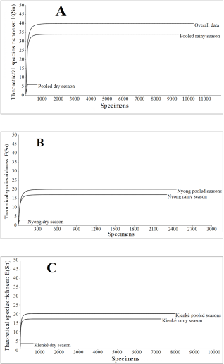
Figure 2. Individual rarefaction curves of the Chromista collections during the dry season and the rainy season in Nyong and Kienke River mouths at both tides.

The highest species richness was recorded in the overall pooled data from both rivers and both seasons (S=40 species; Mg=4.215; d=0.004) (Table 3). Other values of the species richness were found between the two extremes. Individual rarefaction curves approached the plateaus of saturation and for a standard sample of 701.0x10⁵ cells, the pooled data appeared the most species rich (E(S(n=701.0x10⁵))=39±1 species), followed by the distribution in the rainy season (E(S(n=701.0x10⁵))=34±0 species), and the assemblage in the dry season appeared less species rich (E((n=701.0x10⁵))=6±0 species) (Figure 2A). A similar trend was noted in Nyong (E(S(n=131.0x10⁵))=19±1 species for the pooled data; E(S(n=131.0x10⁵))=17±1 species in the rainy season, and E(S(n=131.0x10⁵))=3±0 species in the dry season) (Figure 2B), as well as in Kienke (E(S(n=671.0x10⁵))=20±0 species for the pooled data; E(S(n=671.0x10⁵))=17±0 species in the rainy season, and E(S(n=671.0x10⁵))=3±0 species in the dry season) (Figure 2C).

In each river mouth, the species diversity recorded in rainy season was higher than that recorded in dry season (Table 3). Between the two river mouths, the species diversity recorded in Kienke was significantly higher than that recorded in the Nyong (Table 3). Both river mouths presented a high diversity (Shannon-Weaver’s diversity values were close to the maximum value), a highly even community (Pielou’s values were close to the unity) and a very low dominance by a few species (Berger-Parker index were in all cases inferior to the median value and close to the null value; Table 3).

Pairwise comparison of diversity indexes showed significant differences (Table 3). Considering Chao1 index (non-parametric estimator of the ‘TRUE” species richness), sampling success was maximal (100.0%) (Table 3), suggesting all rare species were collected. Although the rank-frequency plotting of the pooled SAD was close to the Fisher’s log-series model (statistics: α=5.261, x=0.9995, χ²=1.644x10⁴, p=0.0), a fairly weak concave appearance was noted, suggesting absence of a few co-dominants (Figure 3A). The similar shape was noted during the dry season (α=0.8735, x=0.999, χ²=975.7, p=3.4x10^-211; Figure 3B), and during the rainy season (α=4.417, x=0.9995, χ²=1.473x10⁴, p=0.0; Figure 3C). A similar shape was noted during both seasons in Nyong (dry season: α=0.534, x=0.9964, χ²=290.6, p=3.7x10^-65; rainy season: α=2.485, x=0.9989, χ²=4510.0, p=0.0; pooled seasons: α=2.974, x=0.9988, χ²=5764.0, p=0.0; Figure 4), and during both seasons in Kienke (dry season: α=0.4027, x=0.9994, χ²=1844.0, p=0.0; rainy season: α=2.083, x=0.9997, χ²=1.118x10⁴, p=0.0; pooled seasons: α=2.471, x=0.9997, χ²=1.315x10⁴, p=0.0; Figure 5).

Based on the Hill's N₁ and N₂ values, the numbers of abundant species were close to the number of co-dominants (Hill's ratio close to 1) (Table 3), suggesting a low dominance of the assemblages by a few species. On the base of the N₁ diversity number (Table 3) and the rank-abundance plotting (Figures 3, 4 and 5), during the dry season, the recorded three species (Cc. meneghiniana, De. elegans, and Op. cochleare) were simply abundant and co-dominant species in the Nyong River mouth and three other species (Ch. muelleri, Cr. erosa, and Su. linearis) were simply abundant and co-dominants in Kienke (Table 3). During the rainy season, 14 species on the 17 recorded species (82.4%) ( Ac. exiguoides, Am. ovalis, An. sphaerophora, Au. granulate, Ca. noricus, Cm. solea, Co. placentula, Dp. arctica, Fa. construens, Fr. adnata, Gn. mutica, Ha. amphioxys, Pi. cardinaliculus, and Ta. flocculosa) were simply abundant in the Nyong River mouth while 13 species on the 17 recorded species (76.5%) (Cc. stelligera, Ce. hirundinella, De. thermalis, Dp. ovalis, Go. olivaceum, Gn. gigas, Cy. unicorne, Me. granulata, Ni. amphibia, Rh. longiseta, St. astraea, Su. capronii, and Sy. ulna) were abundant in Kienke (Table 3).

Table 3. Matrix of the species richness, diversity, evenness and dominance indexes for the pooled data from both river mouths.

Indices	Nyong River mouths			Kienke River mouths			Both rivers
Indices	I	II	III	I	II	III	I	II	III
A. Richness indexes
n x10⁵ cells	145.8	2,312.5	2,458.3	687.5	7,281.3	7,968.8	833.3	9,593.8	10,427.1
(%)	(1.4)	(22.2)	(23.6)	(6.6)	(69.8)	(76.4)	(8.0)	(92.0)	(100.0)
S (%)	3 (7.5)	17 (42.5)	20 (50.0)	3 (7.5)	17 (42.5)	20 (50.0)	6 (15.0)	34 (85.0)	40 (100.0)
n_maxx10⁵ cells	62.5	385.4	385.4	375.0	1,395.8	1,395.8	375.0	1,395.8	1,395.8
Magalef: Mg	0.401	2.065	2.433	0.306	1.799	2.115	0.743	3.599	4.215
Richness ratio: d = S/n	0.020	0.007	0.008	0.004	0.002	0.003	0.007	0.004	0.004
Chao1	3	17	20	3	17	20	6	34	40
% SE=(S/Chao 1)*100	100.0	100.0	100.0	100.0	100.0	100.0	100.0	100.0	100.0
B. Diversity indexes
Shannon-Weaver H’	1.004	2.612	2.742	0.918	2.530	2.685	1.398	3.102	3.245
H’_max=ln(S)	1.099	2.833	2.996	1.099	2.833	2.996	1.792	3.526	3.689
Simpson’s D	0.388	0.087	0.079	0.438	0.098	0.085	0.309	0.061	0.054
Hill’s N₁ = e^H’	2.730	13.629	15.522	2.503	12.553	14.654	4.048	22.250	25.656
Hill’s N₂ = 1/D	2.579	11.447	12.719	2.286	10.213	11.766	3.236	16.276	18.525
Hill’s ratio N₂/N₁	0.945	0.840	0.819	0.913	0.814	0.803	0.800	0.732	0.722
Rare species: Chao1-N₁	0	3	4	0	4	5	2	12	14
C. Evenness index
Pielou J=(H’/H’_max)	0.914	0.922	0.915	0.835	0.893	0.896	0.780	0.880	0.880
E. Dominance index
I_BP = n_max/n	0.429	0.166	0.156	0.545	0.192	0.175	0.449	0.145	0.134
Pairwise comparisons of diversity indexes (Student t-test)
Comparison	Shannon-Weaver index H’				Simpson’s diversity index
I vs. II	Nyong: t=-45.93; df=119.29; p=5.7x10^-108 * Kienke: t=-76.82; df=961.07; p=0 *				Nyong: t=17.46; df=150.88; p=4.9x10^-38 * Kienke: t=31.72; df=709.56; p=3.5x10^-138 *
Nyong vs. Kienke	Dry season: t=-2.30; df=262.43; p=0.022 * Rainy season: t=-5.28; df=4,285.20; p=1.3x10^-7 * Both seasons: t=-3.62; df=4,316.60; p=3.0x10^-4 *				Dry season: t=2.47; df=273.73; p=0.014 * Rainy season: t=4.46; df=4,615.20; p=8.3x10^-6 * Both seasons: t=2.95; df=4,613.70; p=0.003 *

ns: not significant difference (p≥0.05); *: significant difference (p<0.05); n: sample size; n_max: maximum abundance; S: observed species richness; Mg: Margalef richness index; d: richness ratio; H’: Shannon-Weaver diversity index; H_max: maximum Shannon-Weaver diversity index; D: Simpson’s diversity index; N₁: Hill’s first order diversity number; N₂ = Hill’s second order diversity number; Hill: Hill’s diversity ratio; J: Pielou’s evenness index; I_BP = Berger-Parker dominance index; SE: sampling effort.

Making a total of 17 species (42.5%) in Nyong, 16 species (40.0%) in Kienke, and 33 species (82.5%) in the pooled distribution. Thirty-three species were represented by 9,947.9x10⁵ cells (95.4%) (145.8x10⁵ cells (1.4%) in the dry season in Nyong, 687.5x10⁵ cells (6.6%) in the dry season in Kienke; 2,166.7x10⁵ cells (20.8%) in rainy season in Nyong; 6,947.8x10⁵ cells (66.8%) in rainy season in Kienke). The number rare species was low and they were scarce.

3.2.2. Adjustment of the SADs

Adjustment of SADs to five theoretical models showed a poor quality of fit (Pearson correlation r≤-0.95): dry season in both rivers: r=-0.884, p=0.019, 6 species; dry season in Nyong: r=-0.867, p=0.333, 3 species; dry season in Kienke: r=-0.993, p=0.073, 3 species; rainy season in both rivers: r=-0.828, p=1.5x10^-9, 34 species; rainy season in Nyong: r=-0.912, p=3.5x10^-7, 17 species; rainy season in Kienke: r=-0.913, p=3.3x10^-7, 17 species; pooled seasons in both rivers: r=-0.817, p=1.3x10^-10, 40 species; pooled seasons in Nyong: r=-0.889, p=1.6x10^-7, 20 species; pooled seasons in Kienke: r=-0.896, p=9.6x10^-8, 20 species.

Based on AIC and BIC (Table 4) and SADs (Figures 3, 4 and 5), LN model fitted assemblages with high environmental constants (m’>1), except the pooled assemblage in dry season in both rivers which fitted ZM model. LN model fitted the pooled data with a low m’ value (maximum abundance: n₁=1385.8x10⁵ cells; sample size: n=10,427.1x10⁵ cells; 40 species; deviance=151.06; mean of logarithms of abundance: x=2.206; lognormal variance: σ²=0.192; lognormal standard deviation: σ=0.429; environmental constant: m’=0.493; correction factor: 1.049; corrected model: n_i=33,920.1x10⁵(0.350)^Pi with P_i as probits of species cumulative percentage ranks (Table 4, Figure 3A).

This was the case of the pooled assemblage in the two rivers in the rainy season (n₁=1395.8x10⁵ cells; n=9,593.8x10⁵ cells; 34 species; deviance=107.92; x=2.252; σ²=0.18); σ=0.417; m’=0.522; correction factor: 1.050; corrected model: n_i=33,959.9x10⁵(0.358)^Pi) (Table 4, Figure 3C). ZM model best fitted the pooled assemblage recorded during the dry season in the two river mouths with a low value of the average fractal dimension of the distribution of individuals among species ((1/γ)<1) (deviance=48.44, Q=833.3x10⁵ cells, n₁=375.0x10⁵ cells, 6 species; Gauss-Marquard’s procedure for de determination of the model’s parameters: starting point: x₀=(0; 2)^T; tolerance of the functional value: ε=1.0x10^-10; damping factor: λ₀=100; beta statistic: β=1.340; gamma statistic: γ=1.093; correction factor: 0.787; corrected model: n_i=656.0x10⁵(i+1.340)^-1.093; 1/γ=0.915) (Table 4, Figure 3B). Assemblages in each season and each river fitted the LN model. In Nyong, it was the case of the assemblage in the dry season and the environmental constant was high (m’>1.0) (n₁=62.5x10⁵ cells; n=145.8x10⁵ cells; 3 species; deviance=9.46; x=1.637; σ²=0.076; σ=0.248; m’=1.469; correction factor: 1.011; corrected model: n_i=2,862.8x10⁵(0.046)^Pi cells) (Table 4, Figure 4A), but the environmental constant was low in the rainy season (n₁=385.4x10⁵ cells; n=2,312.5x10⁵ cells; 17 species; deviance=154.94; x=2.029; σ²=0.103; σ=0.309; m’=0.947; correction factor: 1.020; corrected model: n_i=6,296.1x10⁵(0.045)^Pi cells) (Table 4, Figure 4B). LN model fitted the pooled seasons with a low environmental constant (n₁=385.4x10⁵ cells; n=2,458.3x10⁵ cells; 20 species; deviance=53.20; x=1.970; σ²=0.115; σ=0.326; m’=0.853; correction factor: 1.028; corrected model: n_i=6,501.0x10⁵(0.437)^Pi cells (Table 4, Figure 4C).

Download: Download full-size image

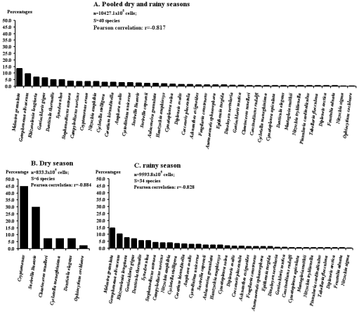
Figure 3. Rank-frequency diagram of the pooled Chromista collection in both river mouths at both tides, showing species in decreasing order of numerical occurrence.

In Kienke, assemblage in dry season fitted the LN model with a low environmental constant (n₁=375.0x10⁵ cells; n=687.5x10⁵ cells; 3 species; deviance=27.93; x=2.256; σ²=0.167; σ=0.397; m’=0.574; correction factor: 0.988; corrected model: n_i=142,622.2x10⁵(0.289)^Pi cells) (Table 4, Figure 5A). A similar result was obtained in rainy season (n₁=1,395.8x10⁵ cells; n=7,281.3x10⁵ cells; 17 species; deviance=94.08; x=2.476; σ²=0.164; σ=0.400; m’=0.566; correction factor: 1.001; corrected model: n_i=56,730.5x10⁵(0.358)^Pi cells) (Table 4, Figure 5B) as well as the pooled assemblage from both seasons (n₁=1,395.8x10⁵ cells; n=7,968.8x10⁵ cells; 20 species; deviance=109.54; x=2.448; σ²=0.162; σ=0.395; m’=0.581; correction factor: 1.008; corrected model: n_i=46,270.4x10⁵(0.367)^Pi cells) (Table 4, Figure 5C).

3.3. Beta Diversity: Dissimilarity Between SADs

Based on the species composition, a few common orders and families were recorded but no species was common to both rivers. In the pooled data, a null level of dissimilarity was detected between the two tides in the dry season (Table 5A) and it was the same in rainy season (Table 5A) as well as between tides in the pooled seasons (Table 5A). However, dissimilarity close to the median value was noted between the data set at high tide in the dry season (HS) and the pooled data at high tide in both rivers (Table 5A).

A low dissimilarity was noted between HS and the overall assemblage (Table 5A). Data at low tide in the dry season showed a null dissimilarity (Table 5A). In the rainy season, a null dissimilarity was noted between high tide and low tide (Table 5A). A low level of dissimilarity was recorded between high tide and the pooled assemble at both tides in rainy season or the pooled assemblage at both tides and both seasons. A high level of dissimilarity was detected when compared to the assemblage at high tide in the pooled both seasons (Table 5A).

The assemblage at low tide showed a high dissimilarity to the assemblage at the pooled tides during the rainy season, to the assemblage at the low tide in the rainy season, or the pooled assemblage in the pooled seasons (Table 5A).

A low dissimilarity was noted between the pooled assemblage in the rainy season and the assemblage at high tide in the rainy season but it was high when compared to the assemblage at low tide in the pooled seasons or to the assemblage at the pooled tides in the pooled seasons (Table 5A). In the pooled data from both seasons, assemblage at high tide showed a null dissimilarity when compared to that noted at low tide. The dissimilarity was low when compared to the pooled tides (Table 5A). In the pooled seasons, low tide showed a high dissimilarity to the pooled tides (Table 5A). In Nyong, dissimilarity was null in both seasons between high and low tides (Table 5B), but in the dry season, it was high between the two tides and the pooled data (Table 5B). It was the same in the rainy season (Table 5B). Combinations in the rainy season showed a null dissimilarity (Table 5B). Comparisons in the pooled seasons showed a low to null dissimilarity during the dry season and high dissimilarities in the rainy season (Table 5B).

Pooled data in rainy season and pooled seasons showed a high dissimilarity (Table 5B). In Kienke, the dissimilarity was null between the two tides in dry season (Table 5C) and it was high when each tide was compared to the pooled data at both tides (Table 5C). Comparisons to data recorded during the rainy season showed a null dissimilarity (Table 5C). High tide in the pooled seasons showed a null dissimilarity when compared to low tide in each season, and the dissimilarity was low when compared to low tide in dry season or to the pooled tides in dry season (Table 5C). But the dissimilarity was high when compared to low tide in the rainy season or to the pooled tides in the same season (Table 5C).

3.4. Correlation Between Species

Twenty-one sample units (12 in Nyong, and nine in Kienke) allowed to detect an overall positive net association (VR>1) in Kienke (Schluter’s Variance ratio: VR=1.795; statistic: W=16.154, df=19, p<0.001) and the pooled assemblage (VR=1.043; W=21.91, df=20, p<0.001).

Download: Download full-size image

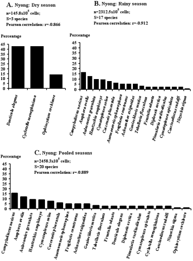
Figure 4. Rank-frequency diagrams of the Chromista collection in the Nyong River mouth at both tides and both seasons, showing species in decreasing order of numerical occurrence.

In Nyong, a negative net association was noted (VR=0.615; W=7.37, df=19, p<0.001). Positive correlation suggested that compared species were mutually tolerant (Table 6). In the pooled assemblage, correlations were positive (Table 6A). Ac. exiguoides was positively associated with Co. placentula (Table 6A). Am. ovalis was positively associated with Cm. apiculata, Cs. rudolfi, and Gn. Mutica. Ca. noricus was positively associated with the useful species Ch. muelleri. Ce. hirundinella was positively correlated with Cr. erosa, and Cc. meneghiniana. Co. placentula was positively correlated with Cm. apiculata, and Gn. mutica (Table 6A). Cs. rudolfi was positively correlated with Fa. construens. Cr. erosa was positively correlated with Cc. meneghiniana, De. elegans, and Rh. longiseta (Table 6A). Cc. meneghiniana was positively correlated with Cc. stelligera (Table 6A). Cm. apiculata was positively correlated with Di. sertularia, and Gn. mutica (Table 6A). Cm. solea was positively correlated with De. elegans, and Ni. sigma (Table 6A). De. elegans was positively correlated with one species (Rh. longiseta) (Table 6A). De. thermalis was positively correlated with Gn. gigas, and Ni. tryblionella. Di. sertularia was positively correlated with Gn. mutica, and Ni. amphibia (Table 6A). Go. olivaceum was positively correlated with Rh. longiseta (Table 6A). Gn. mutica was positively correlated with Pi. cardinaliculus (Table 6A). Ni. amphibia was positively correlated with Ni. tryblionella (Table 6A). Pi. cardinaliculus was positively correlated with St. astraea (Table 6A). In Nyong, correlations were positive (Table 6B). Ac exigoides, Cm. apiculata, Cm. solea, De. elegans and Gn. mutica presented the correlation forms identical to those recorded in the pooled data (Table 6B).

In the case of Am ovalis, the correlations in the pooled data existed in Nyong except that Cs. rudolfi in the pooled data was replaced by Pi. cardinaliculus in Nyong (Table 6B). Ca noricus became positively correlated with Cs. rudolfi instead of Ch. muelleri as it was the case in the pooled data (Table 6B).

Table 4. Akaike Information Criteria (AIC) and Bayesian Information Criteria (BIC) values for the adjusted theoretical models.

SAD model	AIC (BIC) and the best fitted model
	Nyong River mouth			Kienke River mouth
	Dry season 145.8x10⁵ cells 3 species	Rainy season 2,312.5x10⁵ cells 17 species	Pooled data 2,457.3x10⁵ cells 20 species	Dry season 687.5x10⁵ cells 3 species	Rainy season 7,281.3x10⁵ cells 17 species	Pooled data 7,968.8x10⁵ cells 20 species
Broken-Stick (BS)	37.34 (37.34)	299.05 (299.05)	307.81 (307.81)	45.25 (45.25)	245.70 (245.70)	319.54 (319.54)
Log-linear (LL)	34.99 (34.06)	178.43 (179.26)	220.08 (221.08)	58.29 (57.39)	283.22 (284.06)	369.49 (370.48)
Log-normal (LN)	30.32 (28.51) *	153.27 (154.94) *	184.82 (186.81) *	53.04 (51.24) *	226.26 (227.92) *	262.82 (264.81) *
Zipf (Z)	34.21 (32.41)	214.60 (216.27)	252.86 (254.85)	77.00 (75.20)	627.03 (628.70)	688.24 (690.23)
Zipf-Mandelbrot (ZM)	32.32 (29.61)	153.67 (156.17)	186.35 (189.34)	55.04 (52.34)	266.80 (269.30)	347.75 (350.74)

SAD model	AIC (BIC) and the best fitted model
	Pooled rivers
	Dry season n=833.3x10⁵ cells S=6 species	Rainy season n=9,593.8x10⁵ cells S=34 species	Pooled data n=10,427.1x10⁵ cells S=40 species
Broken-Stick (BS)	106.49 (106.49)	529.39 (529.39)	630.97 (630.97)
Log-linear (LL)	93.65 (93.44)	583.01 (584.53)	718.18 (719.87)
Log-normal (LN)	96.72 (96.30)	350.85 (353.90) *	431.95 (435.33) *
Zipf (Z)	109.78 (109.37)	845.13 (848.18)	1,039.65 (1043.03)
Zipf-Mandelbrot (ZM)	92.41 (91.79) *	579.59 (584.17)	NA

AIC: Akaike information criteria; BIC: Bayesian information criteria; * best fitted theoretical model in bold; NA: Not available

Download: Download full-size image

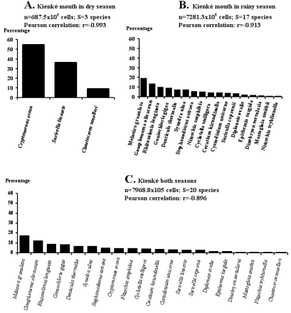
Figure 5. Rank-frequency diagrams of the Chromista collection in the Kienke River mouth at both tides and both seasons, showing species in decreasing order of numerical occurrence.

Table 5. Bray-Curtis dissimilarity values between data sets recorded at two tides during two seasons in the Nyong and Kienke river mouths.

	Dry season			Rainy season			Pooled seasons
	High tide	Low tide	Pooled tides	High tide	Low tide	Pooled tides	High tide	Low tide	Pooled tides
A. Overall data sets
Dry season
High tide	1.000
Low tide	0.0	1.000
Pooled tides	1.000	0.0	1.000
Rainy season
High tide	0.0	0.0	0.0	1.000
Low tide	0.0	0.0	0.0	0.0	1.000
Pooled tides	0.0	0.0	0.0	0.313	0.898	1.000
Pooled seasons
High tide	0.431	0.0	0.431	0.841	0.0	0.295	1.000
Low tide	0.0	0.0	0.0	0.0	1.000	0.898	0.0	1.000
Pooled tides	0.123	0.0	0.123	0.295	0.864	0.966	0.386	0.864	1.000
B. Nyong River mouth
Dry season
High tide	1.000
Low tide	0.0	1.000
Pooled tides	0.727	0.600	1.000
Rainy season
High tide	0.0	0.0	0.0	1.000
Low tide	0.0	0.0	0.0	0.0	1.000
Pooled tides	0.0	0.0	0.0	0.600	0.727	1.000
Pooled seasons
High tide	0.145	0.0	0.137	0.959	0.0	0.585	1.000
Low tide	0.0	0.087	0.082	0.0	0.977	0.715	0.0	1.000
Pooled tides	0.066	0.050	0.113	0.574	0.699	0.969	0.608	0.721	1.000
C. Kienke River mouth
Dry season
High tide	1.000
Low tide	0.0	1.000
Pooled tides	0.706	0.625	1.000
Rainy season
High tide	0.0	0.0	0.0	1.000
Low tide	0.0	0.0	0.0	0.0	1.000
Pooled tides	0.0	0.0	0.0	0.151	0.957	1.000
Pooled seasons
High tide	0.558	0.0	0.453	0.760	0.0	0.144	1.000
Low tide	0.0	0.086	0.081	0.0	0.977	0.936	0.0	1.000
Pooled tides	0.090	0.076	0.159	0.139	0.913	0.955	0.217	0.935	1.000

Table 6. Kendall’s tau correlation recorded between Chromista species in 21 sample units from the Nyong and Kienke River mouths.

Species 1/Species 2		τ (p-value)	Species 1/Species 2		τ (p-value)	Species 1/Species 2		τ (p-value)
A. Overall pooled data from both seasons and both river mouths (n=21)
Ac. exiguoides			Cs. rudolfi			De. thermalis (continued)
	Co. placentula	0.737(3.0x10-6) *		Fa. construens	0.447(0.005) *		Ni. tryblionella	0.425(0.007) *
Am. ovalis			Cr. erosa			Di. sertularia
	Cm. apiculata	0.474 (0.003) *		Cc. meneghiniana	0.445 (0.005) *		Gn. mutica	0.364 (0.021) *
	Cs. rudolfi	0.322 (0.041) *		De. elegans	0.445 (0.005) *		Ni. amphibia	0.568 (3.2x10-4) *
	Gn. mutica	0.742(2.5x10-6) *		Rh. longiseta	0.360 (0.023) *	Go. olivaceum
Ca. noricus			Cc. meneghiniana				Rh. longiseta	0.536 (0.001) *
	Ch. muelleri	0.520 (0.001) *		Cc. stelligera	0.497 (0.002) *	Gn. mutica
Ce. hirundinella			Cm. apiculata				Pi. cardinaliculus	0.645 (4.4x10-5) *
	Cr. erosa	0.431 (0.006) *		Di. sertularia	0.568(3.2x10-4)*	Ni. amphibia
	Cc. meneghiniana	0.378 (0.016) *		Gn. mutica	0.716(5.6x10-6)*		Ni. tryblionella	0.533 (0.001) *
Ch. muelleri			Cm. solea			Pi. cardinaliculus
	Go. olivaceum	0.424 (0.007) *		De. elegans	0.645(4.4x10-5)*		St. astraea	0.424 (0.007) *
	Ni. amphibia	0.592(1.7x10-4) *		Ni. sigma	0.716(5.6x10-6)*
	Rh. longiseta	0.332 (0.035) *	De. elegans
Co. placentula				Rh. longiseta	0.379 (0.016) *
	Cm. apiculata	0.598(1.5x10-4) *	De. thermalis
	Gn. mutica	0.385 (0.015) *		Gn. gigas	0.328 (0.037) *
B. Nyong River mouth (n=12)
Ac. exiguoides			Cs. rudolfi (continued)			Cm. solea
	Co. placentula	0.647 (0.006) *		Fa. construens	0.671 (0.004) *		De. elegans	0.580 (0.013) *
Am. ovalis			Cr. erosa				Ni. sigma	0.725 (0.002) *
	Cm. apiculata	0.580 (0.013) *		De. elegans	0.725 (0.002) *	De. elegans
	Gn. mutica	0.895 (1.3x10^-4) *		Ni. amphibia	0.580 (0.013) *		Rh. longiseta	0.725 (0.002) *
	Pi. cardinaliculus	0.725 (0.002) *		Rh. longiseta	0.474 (0.043) *	Di. sertularia
Ca. noricus			Cc. stelligera				Gn. mutica	0.474 (0.043) *
	Cs. rudolfi	0.580 (0.013) *		Cm. solea	0.725 (0.002) *	Fa. construens
Ce. hirundinella			Cm. apiculata				Ni. amphibia	0.671 (0.004) *
	De. elegans	0.671 (0.004) *		Di. sertularia	0.725 (0.002) *	Gn. mutica
Co. placentula				Gn. mutica	0.725 (0.002) *		Pi. cardinaliculus	0.580 (0.013) *
	Cm. apiculata	0.620 (0.008) *	Cm. apiculata
Cs. rudolfi				Rh. longiseta	0.580 (0.013) *
	Di. sertularia	0.580 (0.013) *
C. Kienke River mouth (n=9)
Am. ovalis			Cs. rudolfi			Di. sertularia
	Cs. rudolfi	1.000 (1.7x10^-4) *		De. thermalis	0.730 (0.006) *		Ni. amphibia	0.548 (0.040) *
	De. thermalis	0.730 (0.006) *	Cr. erosa				Ni. tryblionella	1.000 (1.7x10^-4) *
Ca. noricus				Rh. longiseta	0.553 (0.038) *	Go. olivaceum
	Ch. muelleri	1.000 (1.7x10^-4) *	Cc. stelligera				Rh. longiseta	0.789 (0.003) *
	Ni. amphibia	0.730 (0.006) *		Di. sertularia	0.730 (0.006) *	Ni. amphibia
Ce. hirundinella				Ni. tryblionella	0.730 (0.006) *		Pi. cardinaliculus	0.548 (0.040) *
	St. astraea	0.617 (0.021) *	De. thermalis
Ch. muelleri				Di. sertularia	0.548 (0.040) *
	Ni. amphibia	0.730 (0.006) *		Ni. tryblionella	0.548 (0.040) *

Ce. hirundinella was positively correlated with De. elegans (Table 6B). Co. placentula was correlated with Cm. apiculata (Table 6B). Cs rudolfi was positively correlated with Di. sertularia in Nyong (Table 6B). In the case of Cr. erosa, correlations noted in the pooled data existed in Nyong except Cc. meneghiniana in the pooled data which was replaced by Ni. amphibia in Nyong (Table 6B). The correlations in the pooled data concerning Cc. meneghiniana, Cm. solea, De. thermalis, Go. olivaceum, Ni amphibia, and Pi. cardinaliculus were no longer found in Nyong (Table 6B). Di. sertularia was positively correlated with Gn. mutica (Table 6B).

In Kienke, correlations were positive (Table 6C). Ca noricus was positively correlated with Ni. amphibia (Table 6C). Ce. hirundinella was positively correlated with St. astraea (Table 6C). Ch. muelleri was positively correlated with Ni. amphibia (Table 6C). Cs. rudolfi was positively correlated with De. thermalis (Table 6C). Cr. erosa was positively correlated with Rh. longiseta (Table 6C). Cc. stelligera and De. thermalis were each positively correlated with Di. sertularia and Ni. tryblionella (Table 6C). Di. sertularia was positively correlated with Ni. amphibia and Ni. tryblionella. Go. olivaceum was positively correlated with Rh. longiseta and Ni. amphibia was positively correlated with Pi. cardinaliculus (Table 6C). Other correlations were not significant.

4. Discussion

4.1. Species Richness and Diversity of Chromista

The present study is the first step in an in-depth study of the algae assemblage in Nyong and Kienke (Southern Cameroon), evaluating the place occupied by zoonotic species, or those useful for the nutrition of fish. Collected cells belonged to three phyla, eight classes, 23 orders, 32 genera and 40 species

[20]

species (50.0%) from each river mouth) and no common species was recorded. Melosiraceae was the most collected family (13.4%), followed by Bacillariaceae (12.2%), Surirellaceae (10.8%), Gomphonemataceae (9.6%), Stephanodiscaceae (7.7%), Goniochloridaceae (7.2%), Rhizosoleniaceae (7.0%), Fragilariaceae (6.3%), Cryptomonadaceae3.5%), Ceratiaceae (3.0%), Catenulaceae (2.8), Phytodiniaceae (2.6%), Aulacoseiraceae (2.2%), Diploneidaceae (1.9%), Cocconeidaceae (1.4%), Achnanthaceae (1.2%), Anomoeoneidaceae (1.2%), Rhopalodiaceae (1.2%) while other families were rare and represented each by less than 1.0% of the total collection. The most specious family was Bacillariaceae (15.0% of the total species richness), followed by Surirellaceae (12.5%), Stephanodiscaceae (7.5%). Diploneidaceae and Fragilariaceae were each represented by two species (5.0%). Other families were rare. The high presence and abundance of diatoms is not surprising, as it is the case worldwide, in stagnant or slow flowing waters

[43, 48]

. Based on the information on the recorded contributing diatom species

[64-66]

, the weighed mean sensitivity of taxa (WWS) and the trophic diatom index (TDI) showed that in the studied rivers, the diatom community was in the reference conditions (undisturbed) with no or little alteration of human origin and a low organic pollution (oligotrophic or in mesotrophic state)

[13]	Zalat, A. A., Nitychoruk, J., Chodyka, M., Pidek, I. A., Welc, F. Recent and fossil freshwater diatoms of Poland: taxonomy, distribution and their significance in the environmental reconstruction. Part 1. Coscinodiscophyceae, Mediophyceae and Fragilariophycidae. John Paul II University of Applied Sciences, Biała Podlaska; 2022, pp. 1-306
[14]	Jahn, R., Kusber, W. H., Romero, O. E. Cocconeis pediculus Ehrenberg and C. placentula Ehrenberg var. placentula (Bacillariophyta): Typification and taxonomy. Fottea. 2009, 9(2), 275–288. https://doi.org/10.5507/fot.2009.027 View Article
[15]	Hecky, R. E., Kilhan, P. Diatoms in Alkaline, Saline Lakes: Ecology and Geochemical Implications. Limnology and Oceanography. 1973, 18(1), 53-71. https://doi.org/10.4319/LO.1973.18.1.0053 View Article
[16]	Spaulding, S. A., Potapova, M. G., Bishop, I. W., Lee, S. S., Gasperak, T. S., Jovanovska, E., Edlund, M. B.. Diatoms.org: supporting taxonomists, connecting communities. Diatom Research. 2021, 36(4): 291-304. https://doi.org/10.1080/0269249X.2021.2006790 View Article
[17]	Houk, V.; Klee, R., Tanaka, H. Atlas of freshwater centric diatoms with a brief key and descriptions, Part III, Stephanodiscaceae A, Cyclotella, Tertiarius, Discostella. Fottea. 2010, 10(Supplement), 1–498.
[18]	Krammer, K., Lange-Bertalot, H. Bacillariophyceae, 2nd part: Bacillariaceae, Epithemiaceae, Surirellaceae. In Süsswasserflora von Mitteleuropa, Band 2/2. Ettl, H., Gerloff, J., Heynıg, H., Mollenhauer, D., Eds., Gustav Fischer Verlag, Stuttgart, Germany; 1988, pp. 1-596.
[19]	Krammer, K, Lange-Bertalot, H. Bacillariophyceae, 3. Teil: Centrales, Fragilariaceae, Eunotiaceae. In Süsswasserflora Von Mitteleuropa, Band 2/3. Ettl, H., Gerloff, J., Heynıg, H., Mollenhauer, D., Eds., Gustav Fischer Verlag, Stuttgart, Germany; 1991, pp. 1-596.
[20]	Mohanty, T. R.,•Tiwari, N. K.,•Kumari, S.,•Ray, A.,•Manna, R. K., Bayen, S.,•Roy, S.,•Gupta, S. D.,•Ramteke, M. H.,•Swain, H. S., Bhor, M.,•Das, B. K. Variation of Aulacoseira granulata as an eco pollution indicator in subtropical large river Ganga in India: a multivariate analytical approach. Environmental science and pollution research international. 2022, 29(25), 37498-37512 https://doi.org/10.1007/s11356-021-18096-9 View Article
[21]	Taylor, J. C., Harding, W. R., Archibald, C. G. M. An Illustrated Guide to Some Common Diatom Species from South Africa. WRC Report TT 282/07. Water Research Commission. Gezina, Pretoria, South Africa; 2007, pp. 1-225.
[22]	DeColibus, D. “Tabellaria flocculosa (Roth) Kütz. 1844. In Diatoms of North America”. Available from https://diatoms.org [Accessed 01 March 2024]. View Article

[13-22]

. Values were relatively close to 56.74 reported in Lake Porsuk Dam in Turkey the value

[65]

and 39 to 44.5 reported in the mesotrophic waters of Upper Porsuk Creek Kütahya in Turkey

[67]

. Me. granulata was the most collected (13.4%), followed by Go. olivaceum (9.6%), Rh. longiseta (7.0%), Gn. gigas (6.4%), De. thermalis and Sy. ulna (5.1% respectively), St. astraea (3.9%), Ca. noricus (3.7%), 3.6% respectively for Cr. erosa and Ni. amphibia, Cc. stelligera (3.2%), Ce. hirundinella (3.0%), Am. ovalis (2.8%), Cy. unicorne (2.6%), Su linearis (2.4%), Su. capronii (2.3%), Au. granulata (2.2%), Ha. amphioxys (2.1%). Other species were rare. Twenty-four freshwater species [60.0%: 12 species (30.0%) in Nyong and Kienke respectively] were recorded. Three marine species (7.5%: one species Cs. rudolfi in Nyong and two species Ch. muelleri, and Ep. turgida in Kienke) were recorded. One brackish species (2.5%) (De. thermalis) was noted exclusively in Kienke. Twelve tolerant species (30.0%) (seven (17.5%) in Nyong and five (12.5%) in Kienke) were recorded. Two potentially useful species (the antibiotics pollution detoxifier Ch. muelleri

[21, 24]

and the biofertilizer Epithemia turgida

[23]

) were recorded. One species harmful to the fish was recorded (the bloom forming Ce. hirundinella known as fish-killer species

[31]

) and 37 species (92.5%) of unknown toxigenic status were able to be considered as bioindicators. These waters allowed the development of autotrophic and/or mixotrophic algae species. Useful species were few, lowly abundant and masked by indifferent species which were good resource of the nutrition for aquatic macroinvertebrates and/or macrovertebrates. The recorded harmful species is known to form blooms in stagnant waters of lakes, ponds and reservoirs as well as in slow-moving freshwaters, when water temperatures are warmer than usual

[31]

as the case in Cyanobacteria

[31, 41, 51, 66, 67]

. In the studied mouths, the harmful species found came in addition to the presence of 16 species of toxigenic Cyanobacteria

[41]

, reinforcing the poor quality of the raw waters for human drinking and for fish farming. Non-toxigenic Chromista are abundant and diverse, suggesting either the continuous re-colonization from the tributary rivers, or an appearance of tolerant species adapted to the unstable conditions. Adaptation is well illustrated in tolerant species

[11, 27, 52]

. Twelve tolerant species (30.0%) were recorded (seven (17.5%) in Nyong and five (12.5%) in Kienke) and the two rivers presented a low species richness compared to the situation in other freshwaters. For example, 11 classes, 45 genera and 75 species were reported in Mezam River (Bamenda, Cameroon), amongst which Bacillariophyceae was the most represented class and Naviculaceae was the dominant family

[68]

. A total of 237 epilithic diatom taxa, mostly cosmopolitan, belonging to 39 genera distributed among 25 families were reported in Mfoundi River (Yaounde, Cameroon)

[69]

. It is possible that patterns in Nyong and Kienke depended on local environmental conditions or the sampling methodology and design. Useful species and harmful species were lowly recorded probably because of the regulation of their populations by competing species and/or local natural enemies. Their density could increase if the environmental balance is disrupted due to the climate change force and the growing anthropization actions.

4.2. Community Structure and Functioning Model

Both rivers presented high species diversity, high even community and a low dominance by a few species. In Nyong, the dissimilarity was null in both seasons at high and low tides. In Kienke, the dissimilarity was null at the two tides in dry season and was high when each tide was compared to the pooled tides. The overall assemblage showed a negative global net association in Nyong and a positive net association in Kienke and in the pooled distribution. In each river, assemblage fitted the LN model with low environmental constants (m’<1) except in the dry season in Nyong where m’ was high. Pooled SAD fitted in the dry season, the ZM model with a low fractal dimension of the distribution of individuals among species ((1/γ)<1). LN model describes a community where the majority of species show moderate abundances and it is reported fitting SADs of zooplankton in coastal neritic and estuarine conditions in the Arcachon Bay (France)

[70]

, the freshwater snails at swampy areas in Douala (Cameroon)

[71]

, the Cyanobacteria in Nyong and Kienke

[41]

. Given that nomocenosis are associations of species subject to the influence of the same factors, they characterize evolved or less disturbed environments. ZM model is frequently adapted to evolved communities in natural environments, with a multi-species network structure corresponding to an optimal structure for the circulation of information

[55, 72, 73]

. The pooled assemblage functioned in dry season on the basis of maintaining the complex information network developed at spatio-temporal scales (close to the ecological balance) with a low significant force of regeneration compared to undisturbed freshwaters.

5. Conclusion

The aim of the study was to to establish a baseline of information on the distribution of chromists, in order to evaluate the status and the occurrence of species known as bio-indicators of the aquatic life quality. The studied river mouths presented two useful species and one harmful species to fish. A total of 10,427.1x10⁵ cells belonged to three phyla, eight classes, 23 orders, 32 genera and 40 species. Bacillariophyta was the most collected phylum (71.7%). Melosiraceae was the most collected family (13.4%). Melosira granulata was the most collected species (13.4%). The species diversity was high. Assemblages were highly even and lowly dominated by a few species. Twenty-four freshwater species (60.0%) were recorded. Three marine species (2.4%) were recorded and one brackish specialist was recorded exclusively in Kienke (5.1%). Thirteen tolerant species (32.6%) were recorded. The trophic diatom index showed that the diatoms were in undisturbed conditions. The useful species and the harmful species were rare and exclusively found in Kienke. Species exhibited a positive net association in Kienke and the pooled assemblage from both rivers in the rainy season while it was negative in Nyong. Assemblages fitted LN model with low environmental constants (m’<1) except in dry season in Nyong where m’ was high suggesting that majority of species were moderately abundant (evolved environments). Pooled assemblage in the dry season functioned on the basis of maintaining a complex information network developed at spatio-temporal scales with a low force of regeneration.

Abbreviations

AIC: Akaike Information Criteria

Ac. exiguoides: Achnanthes exiguoides Compère, 1967

Am. ovalis: Amphora ovalis (Kützing) Kützing, 1844

An. sphaerophora: Anomoeoneis sphaerophora E. Pfitzer, 1871

Au. granulata: Aulacoseira granulata (Ehrenberg) Simonsen, 1979

BIC: Bayesian Information Criteria

BS: Broken-Stick Theoretical Model (McArthur’s model)

Ca. noricus: Campylodiscus noricus Ehrenberg ex Kützing, 1844

Cc. meneghiniana: Cyclotella meneghiniana f. meneghiniana Kützing, 1844

Cc. stelligera: Cyclotella stelligera Cleve & Grunow, 1882

Ch. muelleri: Chaetoceros muelleri Lemmermann, 1898

Ce. hirundinella: Ceratium hirundinella (O. F. Müller) Dujardin, 1841

Cm. apiculata: Cymatopleura solar var. apiculata W. Smith, 1853

Cm. solea: Cymatopleura solea var. baicalensis Skvortzow & Meyer, 1928

Co. placentula: Cocconeis placentula Ehrenberg, 1838

Cr. erosa: Cryptomonas erosa Ehrenberg 1832

Cs. rudolfi: Coscinodiscus rudolfi Bachmann, 1938

Cy. unicorne: Cystodinium unicorne G. A. Klebs, 1912

De. elegans: Denticula elegans var. elegans Kützing, 1844

De. thermalis: Denticula thermalis var. fossilis Frenguelli, 1936

Di. sertularia: Dinobryon sertularia Ehrenberg, 1834

Dp. arctica: Diploneis arctica (Lange–Bertalot) Lange–Bertalot & A. Fuhrmann, 2016

Dp. ovalis: Diploneis ovalis var. pumila (Grunow) Cleve, 1894

Ep. turgida: Epithemia turgida var. turgida (Ehrenberg) Kützing, 1844

Fa. construens: Fragilaria construens f. construens (Ehrenberg) Grunow, 1862

Fr. adnata: Frustulia adnata Kützing, 1833

Gn. gigas: Goniochloris gigas Bourrelly

Gn. mutica: Goniochloris mutica (A. Braun) Fott, 1960

Go. olivaceum: Gomphonema olivaceum (Lyngbye) Desmazières, 1825

Ha. amphioxys: Hantzschia amphioxys (Ehrenberg) Grunow, 1880

LL: Lognear

LN: Lognormal

Ma. smithii: Mastogloia smithii Thwaites ex W. Smith, 1856

Me. granulata: Melosira granulata var. angustissima Otto Müller, 1899

Ni. amphibia: Nitzschia amphibia Grunow, 1862

Ni. sigma: Nitzschia sigma (Kützing) W. Smith, 1853

Ni. tryblionella: Nitzschia tryblionella Hantzsch, 1860

Op. cochleare: Ophiocytium cochleare (Eichwald) A. Braun 1855

Pi. cardinaliculus: Pinnularia cardinaliculus var. ceylonica Skvortzow, 1930

Rh. longiseta: Rhizosolenia longiseta O. Zacharias, 1893

St. astraea: Stephanodiscus astraea (Ehrenberg) Grunow, 1880

Su. capronii: Surirella capronii Brébisson & Kitton, 1869

Su linearis: Surirella linearis f. kolhapurensis Sarode & Kamat, 1984

Sy. ulna: Synedra ulna (Nitzsch) Ehrenberg, 1832

SAD(s): Species Abundance Distribution(s)

sp.: species plurimae

Ta. flocculosa: Tabellaria flocculosa (Roth) Kützing, 1844

VR: Variance Ratio of Schluter

Z: Zipft

ZM: Zipft-Mandelbrot

Acknowledgments

The authors acknowledge Mrs. Fumdjum Marie for financing laboratory analyzes and the staff the micro-algae laboratory of the Specialized Center for Research on Marine Ecosystems at Kribi (AquaSol service) for the hospitality. They thank canoeists for making their canoe available, elders of Laboratory of Biotechnology and Environment (University of Yaounde 1) and the Laboratory of Biology of Animal Organisms (University of Douala) for assistance in species identification, data analysis and the manuscript preparation.

Author Contributions

Christelle Chimene Mokam: Conceptualization, Data curation, Formal Analysis, Investigation, Methodology, Writing – original draft, Writing – review & editing

Andrea Sarah Kenne Toukem: Software, Formal Analysis, Writing – original draft

Christian Dongmo Teufack: Investigation, Methodology

Fabien Tresor Amougou Dzou: Investigation, Methodology

Sedrick Junior Tsekane: Software, Formal Analysis, Writing – original draft

Mohammadou Moukhtar: Formal Analysis, Writing – original draft

Auguste Pharaon Mbianda: Software, Formal Analysis, Writing – original draft

Martin Kenne: Conceptualization, Resources, Data curation, Software, Formal Analysis, Supervision, Funding acquisition, Validation, Writing – original draft, Project administration, Writing – review & editing

Funding

The Cameroonian Ministry of Higher Education provided funds through the research support program.

Data Availability Statement

The data supporting the outcome of this research work has been reported in this manuscript. They are available from the corresponding author upon reasonable request.

Conflicts of Interest

The authors declare no conflicts of interest.

References

[1]	Guiry, M. D. How many species of algae are there? A reprise. Four kingdoms, 14 phyla, 63 classes and still growing. Journal of Phycology. 2024, 00, 1–15. https://doi.org/10.1111/jpy.13431
[2]	Cavalier-Smith, T. Eukaryote kingdoms: seven or nine? Biosystems. 1981, 14, 461-481. https://doi.org/10.1016/0303-2647(81)90050-2
[3]	Cavalier-Smith, T. Early evolution of eukaryote feeding modes, cell structural diversity, and classification of the protozoan phyla Loukozoa, Sulcozoa, and Choanozoa. European Journal of Protistology. 2013, 49, 115-178. https://doi.org/10.1016/j.ejop.2012.06.001
[4]	Cavalier-Smith, T. Kingdom Chromista and its eight phyla: a new synthesis emphasising periplastid protein targeting, cytoskeletal and periplastid evolution, and ancient divergences. Protoplasma. 2018, 255, 297-357. https://doi.org/10.1007/s00709-017-1147-3
[5]	Aubert, D. Une nouvelle mégaclassification pragmatique du vivant. Médecine/Sciences. 2016, 32, 497-499. https://doi.org/10.1051/medsci/20163205017
[6]	Johnson, L. R., John, D. M., Whitton, B. A., Brook, A. J. Phylum Xanthophyta (Tribophyta) (Yellow-Green Algae). In The Freshwater Algal Flora of the British Isles: An Identification Guide to Freshwater and Terrestrial Algae, Second Edition, Johnson, L. R., Ed., Cambridge University Press. 2021, pp. 318-345. https://doi.org/10.1017/CHOL9781108784122.019
[7]	Guiry, M. D. How many species of algae are there? Journal of Phycology. 2012, 48(5), ‎1057–1063. https://doi.org/10.1111/j.1529-8817.2012.01222.x
[8]	Ruggiero, M. A., Gordon, D. P., Orrell, T. M., Bailly, N., Bourgoin, T., Brusca, R. C., Cavalier-Smith, T., Guiry, M. D., and, Kirk, P. M. A Higher Level Classification of All Living Organisms. PLoS ONE. 2015, 10(4), e0119248. https://doi.org/10.1371/journal.pone.01192489
[9]	Hagen, J. Five Kingdoms, More or Less: Robert Whittaker and the Broad Classification of Organisms. BioScience, 2012, 62. 67-74. https://doi.org/10.1525/bio.2012.62.1.11
[10]	Integrated Taxonomic Information System. “Chromista". Available from www.itis.gov, CC0). [Accessed 29 Febuary 2024], https://doi.org/10.5066/F7KH0KBK
[11]	DiatomBase. “Chromista”. Available from https://diatombase.org [Accessed 26 Febuary 2024].
[12]	Bloch, K., Vardi, P. Microalgae as photosynthetic oxygen generators for pollution control, life support systems and medicine, In Algae: Nutrition, Pollution Control and Energy Sources, Hagen, K. N., Ed., Nova Science Publishers, Inc. Tel-Aviv University, Petah Tikva, Israel; 2009, pp. 3-11.
[13]	Zalat, A. A., Nitychoruk, J., Chodyka, M., Pidek, I. A., Welc, F. Recent and fossil freshwater diatoms of Poland: taxonomy, distribution and their significance in the environmental reconstruction. Part 1. Coscinodiscophyceae, Mediophyceae and Fragilariophycidae. John Paul II University of Applied Sciences, Biała Podlaska; 2022, pp. 1-306
[14]	Jahn, R., Kusber, W. H., Romero, O. E. Cocconeis pediculus Ehrenberg and C. placentula Ehrenberg var. placentula (Bacillariophyta): Typification and taxonomy. Fottea. 2009, 9(2), 275–288. https://doi.org/10.5507/fot.2009.027
[15]	Hecky, R. E., Kilhan, P. Diatoms in Alkaline, Saline Lakes: Ecology and Geochemical Implications. Limnology and Oceanography. 1973, 18(1), 53-71. https://doi.org/10.4319/LO.1973.18.1.0053
[16]	Spaulding, S. A., Potapova, M. G., Bishop, I. W., Lee, S. S., Gasperak, T. S., Jovanovska, E., Edlund, M. B.. Diatoms.org: supporting taxonomists, connecting communities. Diatom Research. 2021, 36(4): 291-304. https://doi.org/10.1080/0269249X.2021.2006790
[17]	Houk, V.; Klee, R., Tanaka, H. Atlas of freshwater centric diatoms with a brief key and descriptions, Part III, Stephanodiscaceae A, Cyclotella, Tertiarius, Discostella. Fottea. 2010, 10(Supplement), 1–498.
[18]	Krammer, K., Lange-Bertalot, H. Bacillariophyceae, 2nd part: Bacillariaceae, Epithemiaceae, Surirellaceae. In Süsswasserflora von Mitteleuropa, Band 2/2. Ettl, H., Gerloff, J., Heynıg, H., Mollenhauer, D., Eds., Gustav Fischer Verlag, Stuttgart, Germany; 1988, pp. 1-596.
[19]	Krammer, K, Lange-Bertalot, H. Bacillariophyceae, 3. Teil: Centrales, Fragilariaceae, Eunotiaceae. In Süsswasserflora Von Mitteleuropa, Band 2/3. Ettl, H., Gerloff, J., Heynıg, H., Mollenhauer, D., Eds., Gustav Fischer Verlag, Stuttgart, Germany; 1991, pp. 1-596.
[20]	Mohanty, T. R.,•Tiwari, N. K.,•Kumari, S.,•Ray, A.,•Manna, R. K., Bayen, S.,•Roy, S.,•Gupta, S. D.,•Ramteke, M. H.,•Swain, H. S., Bhor, M.,•Das, B. K. Variation of Aulacoseira granulata as an eco pollution indicator in subtropical large river Ganga in India: a multivariate analytical approach. Environmental science and pollution research international. 2022, 29(25), 37498-37512 https://doi.org/10.1007/s11356-021-18096-9
[21]	Taylor, J. C., Harding, W. R., Archibald, C. G. M. An Illustrated Guide to Some Common Diatom Species from South Africa. WRC Report TT 282/07. Water Research Commission. Gezina, Pretoria, South Africa; 2007, pp. 1-225.
[22]	DeColibus, D. “Tabellaria flocculosa (Roth) Kütz. 1844. In Diatoms of North America”. Available from https://diatoms.org [Accessed 01 March 2024].
[23]	Lowe, R. “Epithemia turgida. In Diatoms of North America”. Available from https://diatoms.org/species/epithemia_turgida [Accessed 22 January 2024].
[24]	Mojiri, A, Baharlooeian, M, Zahed M. A. The Potential of Chaetoceros muelleri in Bioremediation of Antibiotics: Performance and Optimization. International Journal of Environmental Research in Public Health. 2021, 22, 18(3), 977. https://doi.org/10.3390/ijerph18030977
[25]	Sivonen, K. Cyanobacterial toxins and toxin production. Phycologia. 1996, 35, 12-24. https://doi.org/10.2216/I0031-8884-35-6S-12.1
[26]	Mankiewicz, J., Tarczynska, M., Walter, Z., Zalewski, M. Natural Toxins from Cyanobacteria, Acta Biologica Cracoviensia Series Botanica. 2003, 45(2), 9-20.
[27]	WHO (World Health Organization). Chapter 8 – Algae and Cyanobacteria in Freshwater. In Guidelines for safe recreational waters. Volume 1 – Coastal and fresh waters. Geneva, Switzerland; 2003, pp. 136-158.
[28]	Zanchett, G., Oliveira-Filho, E. Cyanobacteria and Cyanotoxins: From Impacts on Aquatic Ecosystems and Human Health to Anticarcinogenic Effects. Toxins. 2013, 5, 1896-917. https://doi.org/10.3390/toxins5101896
[29]	Rastogi, R. P., Madamwar, D., Incharoensakdi, A. Bloom Dynamics of Cyanobacteria and Their Toxins: Environmental Health Impacts and Mitigation Strategies. Frontiers in Microbiology. 2015, 6, 1254. https://doi.org/10.3389/fmicb.2015.01254
[30]	Beasley, V. R. Harmful Algal Blooms (Phycotoxins). In Reference Module in Earth Systems and Environmental Sciences, Elsevier Inc. 2019. https://doi.org/10.1016/B978-0-12-409548-9.11275-8
[31]	Nicholls, K. H., Kennedy, W., Hammett, C. A fish-kill in Heart Lake, Ontario, associated with the collapse of a massive population of Ceratium hirundinella (Dinophyceae). Freshwater Biology. 1980, 10, 553-561. https://doi.org/10.1111/j.1365-2427.1980.tb01231.x
[32]	Caturao, R. D. Harmful and toxic algae. In Health Management in Aquaculture (2nd edition). Aquaculture Department, Southeast Asian Fisheries Development Center, Lio-Po G. D. & Inui, Y., Eds., Tigbauan, Iloilo, Philippines; 2010, pp. 170-182.
[33]	Magray, A. R., Lone, S. A., Ganai, B. A., Ahmad, F., Hafeez, S. The first detection and in vivo pathogenicity characterization of Saprolegnia delica from Kashmir Himalayas. Aquaculture. 2021, 542, 736876. https://doi.org/10.1016/j.aquaculture.2021.736876
[34]	Raghukumar, S. Ecology of the marine protists, the Labyrinthulomycetes (Thraustochytrids and Labyrinthulids). European Journal of Protistology. 2022, 38(2), 127-145. https://doi.org/10.1078/0932-4739-00832
[35]	Brummett, R. E., Nguenga, D., Tiotsop, F., Abina, J.-C... The commercial fishery of the middle Nyong River, Cameroon: productivity and environmental threats. Smithiana Bulletin. 2010, 11, 3-16.
[36]	Olivry, J. C. Monographie hydrologique. Fleuves et rivières du Cameroun. Ministère de l’Enseignement Supérieur et de la Recherche Scientifique au Cameroun - Institut Français de Recherche Scientifique pour le Developpement en Coopération/ (MESRES-ORSTOM). Collection "Monographies Hydrologiques ORSTOM" No 9, Paris. 1986, pp. 1-781.
[37]	Dounias, E., Cogels, S., Mvé Mbida, S., Carrière, S. The safety net role of inland fishing in the subsistence strategy of multiactive forest dwellers in southern Cameroon. Revue d’Ethnoécologie. 2016, 10, 11-56.
[38]	Mama, A. C., Mbeng, O., Dongmo, C., Ohondja, A. Tidal Variations and its impacts on the abundance and diversity of phytoplankton in the Nyong estuary of Cameroon. Journal of Multidisciplinary Engineering Science and Technology. 2016, 3(1), 3159-3199.
[39]	Mama, A. C., Youbouni Ghepdeu, G. F., Ngoupayou Ndam, J. R., Bonga, M. D., Onana, F. M., Onguene, R. Assessment of water quality in the lower Nyong estuary (Cameroon, Atlantic Coast) from environmental variables and phytoplankton communities’ composition. African Journal of Environmental Science and Technology. 2018, 12(6), 198-208. https://doi.org/10.5897/AJEST2017.2454
[40]	Essomba Biloa, R. E., Noah Ewoti, O. V., Tuekam Kayo, R. P., Sob Nangou, P. B., Tchakounté, S., Onana, F. M., Nyamsi Tchatcho, N. L., Zebaze Togouet S. H. Zooplankton Dynamics of the Kienke Estuary (Kribi, South Region of Cameroon): Importance of Physico-Chemical Parameters. Open Journal of Ecology. 2021, 11, 837-869. https://doi.org/10.4236/oje.2021.1112051
[41]	Mokam, C. C., Kenne Toukem, A. S., Dongmo Teufack, C., Amougou Dzou, F. T., Tsekane, S. J., Moukhtar, M., Mbianda, A. P., Kenne M. Water Quality, Biodiversity and Abundance of Blue-Green Algae in Nyong and Kienke River Mouths (South-Cameroon). International Journal of Ecotoxicology and Ecobiology. 2024, 9(1), 1-27. https://doi.org/10.11648/j.ijee.20240901.11
[42]	Climate-Data.org. Climat Kribi (Cameroun). Available from https://fr.climate-data.org [Accessed 22 January 2024].
[43]	Compère, P. Algues de la région du Lac Tchad. IV: Diatomophycées. Cahier ORSTOM, série. Hydrohiologie. 1975, 9(4), 205-290.
[44]	Carty, S. Freshwater Dinoflagellates of North America. Comstock Publishing Associates, Cornell University Press. Ithaca, New York, USA. 2014, pp. 280. https://doi.org/10.7591/9780801470370
[45]	Olenina, I., Hajdu, S., Edler, L., Andersson, A., Wasmund, N., Busch, S., Göbel, J., Gromisz, S., Huseby, S., Huttunen, M., Jaanus, A., Kokkonen, P., Ledaine, I., Niemkiewicz, E.. Biovolumes and size-classes of phytoplankton in the Baltic Sea HELCOM Balt. Sea Environ. Proc. No. 106. 2006, pp. 1-144.
[46]	Bellinger, E. G., Sigee, D. C. Freshwater Algae. Identification and Use as Bioindicators. Wiley-Blackwell, Hoboken, USA. 2010, pp. 1-271.
[47]	Jahn, R., Kusber, W.-H. A Key to Diatom Nomenclature. Diatom Research. 2009, 24(1), 101-111. http://dx.doi.org/10.1080/0269249X.2009.9705785
[48]	DREAL (Direction Régionale de l’Environnement, de l’Aménagement et du logement d’Occitanie). "Atlas des Diatomées de l’ex partie Languedoc-Roussillon. Languedoc Roussillon". Available from https://www.occitanie.developpement-durable.gouv.fr/atlas-des-diatomees-de-l-ex-partie-languedoc-a25336.html [Accessed 22 January 2021].
[49]	Sonneman, J. A., Sincock, A., Fluin, J., Reid, M., Newall, P., Tibby, J., Gell, P. An Illustrated Guide to Common Stream Diatom Species from Temperate Australia. Cooperative Research Centre for Freshwater Ecology. Identification guide n°33. Land & Water Resources Research & Development Corporation. 2nd Australian Algal Workshop, Adelaide University, 17-19th April, 2000, pp. 1-166.
[50]	Kumar, D. S., Maurya, O. N. Floristic Survey of Algae in Vikramsila Gangetic Dolphin Sanctuary, Bihar (India). Nelumbo. 2015, 57, 124-134. https://doi.org/10.20324/nelumbo/v57/2015/87116
[51]	WoRMS (World Register of Marine Species). “Chromista”. Available from https://www.marinespecies.org/aphia.php?p=taxdetails&id=7 at VLIZ. [Accessed 06 February 2024].
[52]	Guiry, M. D., Guiry, G. M. 2024. “Kingdom Chromista Cavalier-Smith 1981”. AlgaeBase. World-wide electronic publication, University of Galway, Ireland. Available from https://www.algaebase.org [Accessed 28 February 2024].
[53]	Wilson, J. B. Methods for fitting dominance/diversity curves. Journal of Vegetation Science. 1991, 2(1), 35-46. https://doi.org/10.2307/3235896
[54]	Iganaki, H. Mise au point de la loi de Motomura et essai d’une ecologie ́evolutive. Vie et Milieu. 1967, 18, 153-166.
[55]	Li, W. Zipf's Law Everywhere. Glottometrics. 2002, 5, 14-21.
[56]	Zipf, G. K.,. Human Behavour and the Principle of Least Effort: An introduction to human ecology. 2nd edition, Hafner, New York, NY, USA. 1965, pp. 1-573.
[57]	Le, D.-H., Pham, C.-K., Nguyen, T. T. T., Bui, T. T. Parameter extraction and optimization using Levenberg-Marquardt algorithm,. In Proceedings of 2012 IEEE conference. Fourth International Conference on Communications and Electronics (ICCE), Hanoi University of Science and Technology, Hanoi (Vietnam), 2022; pp. 434-437. https://doi.org/10.1109/CCE.2012.6315945
[58]	Frontier, S. Applications of Fractal Theory to Ecology. In Developments in Numerical Ecology., Legendre P., Legendre, L., Eds., NATO ASI Series book series (volume 14). Springer, Berlin, Heidelberg. 1987, pp. 335-378.
[59]	Bach, P., Amanieu, M., Lam-Hoai, T., Lasserre, G. Application du modele de distribution d'abondance de Mandelbrot a l'estimation des captures dans l'étang de Thau. Journal du Conseil/Conseil Permanent International pour l'Exploration de la Mer. 1988, 44, 235-246. https://doi.org/10.1093/icesjms/44.3.235
[60]	Murthy, Z. V. P. Nonlinear Regression: Levenberg-Marquardt Method, In Encyclopedia of Membranes, Drioli, E., Giorno L., Eds., Springer-Verlag, Berlin, Heidelberg, 2014, pp. 1-3.
[61]	Ludwig, J. A., Raynolds, J. F. Statistical Ecology. John Wiley & Sons, New York, USA. 1988, pp. 1-337.
[62]	Friedman, N. & Potapova, M. “Pinnularia cardinaliculus”. In Diatoms of North America. Available from https://diatoms.org [Accessed 22 January 2024].
[63]	Lange-Bertalot, H., Fuhrmann, A. Contribution to the genus Diploneis (Bacillariophyta): Twelve species from Holarctic freshwater habitats proposed as new to science. Fottea. 2016, 16(2), 157–183. https://doi.org/10.5507/fot.2015.027
[64]	Kelly, M. G., Whitton, B. A.. The trophic diatom index: a new index for monitoring eutrophication in rivers. Journal of Applied Phycology. 1995, 7, 433-444. https://doi.org/10.1007/BF00003802
[65]	Tokatli, C. Evaulation of water quality by using trophic diatom index: example of Porsuk Dam Lake. Journal of Applied Biological Sciences 2013, 7(1), 01-04.
[66]	Kelly, M. G., Adams, C., Graves, A. C., Jamieson, J., Krokowski, J., Lycett, E. B., Murray-Bligh, J., Pritchard, S., Wilkins, C. The trophic diatom index: A User’s manual. Revised Edition. R & D technical Report E2/TR2. Environment Agency, Almondsbury, Bristol, BS32 4UD; 2001, pp. 1-135.
[67]	Solak, C., N. The Application of Diatom Indices in the Upper Porsuk Creek Kütahya – Turkey. Turkish Journal of Fisheries and Aquatic Sciences. 2011, 11, 31-36. https://doi.org/10.4194/trjfas.2011.0105
[68]	Ndjouondo, G. P., Nwamo, R. D., Choula Tegantchouang, F. Diversity and Structure of Microalgae in the Mezam River (Bamenda, Cameroon). African Journal of Environment and Natural Science Research. 2023, 6(1), 19-35. https://doi.org/10.52589/AJENSR-O9H3LUP0
[69]	Menye, D. É., Zébazé Togouet, S. H., Menbohan, S. F., Kemka, N., Nola, M., Boutin, C., Nguetsop, V. F., Djaouda, M., Njiné, T. Bio-écologie des diatomées épilithiques de la rivière Mfoundi (Yaoundé, Cameroun): diversité, distribution spatiale et influence des pollutions organiques. Revue des sciences de l’eau/Journal of Water Science. 2012, 25(3), 203–218. https://doi.org/10.7202/1013103ar
[70]	Castel, J., Courties, C. Composition and differential distribution of zooplankton in Arcachon Bay. Journal of Plankton Research. 1982, 4(3), 417-433. https://doi.org/10.1093/plankt/4.3.417
[71]	Kenne, E. L., Yetchom-Fondjo, J. A., Moumite, M. B., Tsekane, S. J., Ngamaleu-Siewe, B., Fouelifack-Nintidem, B., Biawa-Kagmegni, M., Tuekam Kowa, P. S., Fantio, R. M., Yomon, A. K., Kentsop-Tsafong, R. M., Dim-Mbianda, A. M., Kenne M. Species composition and diversity of freshwater snails and land snails at the swampy areas and streams edges in the urban zone of Douala, Cameroon. International Journal of Biological and Chemical Sciences. 2021, 15(4), 1297-1324. https://dx.doi.org/10.4314/ijbcs.v15i4.2
[72]	Shea, K., Chesson, P. Community ecology theory as a framework for biological invasions. Trends in Ecology and Evolution. 2002, 17(4), 170-176. https://doi.org/10.1016/S0169-5347(02)02495-3
[73]	Ferreira, F. C., Petrere-Jr., M. Comments about some species abundance patterns: classic, neutral, and niche partitioning models, Brazilian Journal of Biology, 2008, 68(4, Suppl.), 1003-1012. https://doi.org/10.1590/S1519-69842008000500008

Cite This Article

Plain Text BibTeX RIS

APA Style

Mokam, C. C., Toukem, A. S. K., Teufack, C. D., Dzou, F. T. A., Tsekane, S. J., et al. (2024). Biodiversity and the Community Structure of Chromista Cavalier-Smith, 1981 in Nyong and Kienke River Mouths (South-Cameroon). International Journal of Ecotoxicology and Ecobiology, 9(1), 28-55. https://doi.org/10.11648/j.ijee.20240901.12

Copy | Download

ACS Style

Mokam, C. C.; Toukem, A. S. K.; Teufack, C. D.; Dzou, F. T. A.; Tsekane, S. J., et al. Biodiversity and the Community Structure of Chromista Cavalier-Smith, 1981 in Nyong and Kienke River Mouths (South-Cameroon). Int. J. Ecotoxicol. Ecobiol. 2024, 9(1), 28-55. doi: 10.11648/j.ijee.20240901.12

Copy | Download

AMA Style

Mokam CC, Toukem ASK, Teufack CD, Dzou FTA, Tsekane SJ, et al. Biodiversity and the Community Structure of Chromista Cavalier-Smith, 1981 in Nyong and Kienke River Mouths (South-Cameroon). Int J Ecotoxicol Ecobiol. 2024;9(1):28-55. doi: 10.11648/j.ijee.20240901.12

Copy | Download

@article{10.11648/j.ijee.20240901.12,
  author = {Christelle Chimene Mokam and Andrea Sarah Kenne Toukem and Christian Dongmo Teufack and Fabien Tresor Amougou Dzou and Sedrick Junior Tsekane and Mohammadou Moukhtar and Auguste Pharaon Mbianda and Martin Kenne},
  title = {Biodiversity and the Community Structure of Chromista Cavalier-Smith, 1981 in Nyong and Kienke River Mouths (South-Cameroon)
},
  journal = {International Journal of Ecotoxicology and Ecobiology},
  volume = {9},
  number = {1},
  pages = {28-55},
  doi = {10.11648/j.ijee.20240901.12},
  url = {https://doi.org/10.11648/j.ijee.20240901.12},
  eprint = {https://article.sciencepublishinggroup.com/pdf/10.11648.j.ijee.20240901.12},
  abstract = {A survey was undertaken from March to June 2014 on the biodiversity and the community structure of Chromista Cavalier-Smith, 1981 in Nyong and Kienke River mouths (South-Cameroon). In each river, raw waters were collected from upstream to downstream at four sites. Cells were counted using the Malassez cells procedure and species were identified. A total of 10427.1x105 cells corresponded to three phyla, eight classes, 23 orders, 32 genera and 40 species (24 freshwater species (60.0% of total species richness and total collection respectively), three marine species (7.5% and 2.4% of the total species richness; and total collection respectively), and one brackish water specialist in Kienke (2.5% and 5.1%), 13 tolerant species (32.5% and 32.6%)). The trophic diatom index revealed undisturbed conditions with no or little alteration of human origin and a low organic pollution (oligotrophic or mesotrophic state) (Nyong: TDI=52.7; Kienke: TDI=69.7; pooled assemblage: TDI=65.0). A low species richness was detected (richness ratio in Nyong: d=0.008; Kienke: d=0.003; pooled rivers: d=0.004), a high species diversity (Shannon index close to maximum) (Nyong: H’=2.742 and H’max=2.996; Kienke: H’=2.685 and H’max=2.996; pooled rivers: H’=3.245 and H’max=3.689), a very low dominance by a few species (Berger-Parker index close to 0) (Nyong: IBP=0.156; Kienke: IBP=0.175; pooled rivers: IBP=0.134), and Hill’s ratio were close to 1 (Nyong: Hill=0.819; Kienke: Hill=0.803; pooled rivers: Hill=0.722). The community was highly even with a high value of the Pielou’s evenness close to 1 (Nyong: J=0.915; Kienke: J=0.896; pooled rivers: J=0.880). Two useful species and one harmful species to fish were rare in Kienke. Species exhibited in Kienke and pooled data in rainy season, a positive global net association while it was negative in Nyong. Assemblage fitted Preston’s model in Nyong with a high environmental constant in the dry season (m’=1.469), low constant in the rainy season (m’=0.947) and the pooled seasons (m’=0.853). In Kienke constants were low (dry season: m’=0.574; rainy season: m’=0.566; pooled seasons: m’=0.581) suggesting a evolved community in less disturbed environments where the majority of species showed moderate abundances. In the dry season, the pooled assemblage functionned on the basis of maintaining a complex information network (close to ecological balance) developed at spatio-temporal scales (ZM model) and it presented a low force of regeneration (fractal dimension of the distribution of individuals among species (1/γ)=0.925<1). The evolved oligotrophic state (close to natural balance) of the chromists’ community should be preserved and protected and the studied rivers classified as reference.
},
 year = {2024}
}

Copy | Download

TY  - JOUR
T1  - Biodiversity and the Community Structure of Chromista Cavalier-Smith, 1981 in Nyong and Kienke River Mouths (South-Cameroon)

AU  - Christelle Chimene Mokam
AU  - Andrea Sarah Kenne Toukem
AU  - Christian Dongmo Teufack
AU  - Fabien Tresor Amougou Dzou
AU  - Sedrick Junior Tsekane
AU  - Mohammadou Moukhtar
AU  - Auguste Pharaon Mbianda
AU  - Martin Kenne
Y1  - 2024/04/02
PY  - 2024
N1  - https://doi.org/10.11648/j.ijee.20240901.12
DO  - 10.11648/j.ijee.20240901.12
T2  - International Journal of Ecotoxicology and Ecobiology
JF  - International Journal of Ecotoxicology and Ecobiology
JO  - International Journal of Ecotoxicology and Ecobiology
SP  - 28
EP  - 55
PB  - Science Publishing Group
SN  - 2575-1735
UR  - https://doi.org/10.11648/j.ijee.20240901.12
AB  - A survey was undertaken from March to June 2014 on the biodiversity and the community structure of Chromista Cavalier-Smith, 1981 in Nyong and Kienke River mouths (South-Cameroon). In each river, raw waters were collected from upstream to downstream at four sites. Cells were counted using the Malassez cells procedure and species were identified. A total of 10427.1x105 cells corresponded to three phyla, eight classes, 23 orders, 32 genera and 40 species (24 freshwater species (60.0% of total species richness and total collection respectively), three marine species (7.5% and 2.4% of the total species richness; and total collection respectively), and one brackish water specialist in Kienke (2.5% and 5.1%), 13 tolerant species (32.5% and 32.6%)). The trophic diatom index revealed undisturbed conditions with no or little alteration of human origin and a low organic pollution (oligotrophic or mesotrophic state) (Nyong: TDI=52.7; Kienke: TDI=69.7; pooled assemblage: TDI=65.0). A low species richness was detected (richness ratio in Nyong: d=0.008; Kienke: d=0.003; pooled rivers: d=0.004), a high species diversity (Shannon index close to maximum) (Nyong: H’=2.742 and H’max=2.996; Kienke: H’=2.685 and H’max=2.996; pooled rivers: H’=3.245 and H’max=3.689), a very low dominance by a few species (Berger-Parker index close to 0) (Nyong: IBP=0.156; Kienke: IBP=0.175; pooled rivers: IBP=0.134), and Hill’s ratio were close to 1 (Nyong: Hill=0.819; Kienke: Hill=0.803; pooled rivers: Hill=0.722). The community was highly even with a high value of the Pielou’s evenness close to 1 (Nyong: J=0.915; Kienke: J=0.896; pooled rivers: J=0.880). Two useful species and one harmful species to fish were rare in Kienke. Species exhibited in Kienke and pooled data in rainy season, a positive global net association while it was negative in Nyong. Assemblage fitted Preston’s model in Nyong with a high environmental constant in the dry season (m’=1.469), low constant in the rainy season (m’=0.947) and the pooled seasons (m’=0.853). In Kienke constants were low (dry season: m’=0.574; rainy season: m’=0.566; pooled seasons: m’=0.581) suggesting a evolved community in less disturbed environments where the majority of species showed moderate abundances. In the dry season, the pooled assemblage functionned on the basis of maintaining a complex information network (close to ecological balance) developed at spatio-temporal scales (ZM model) and it presented a low force of regeneration (fractal dimension of the distribution of individuals among species (1/γ)=0.925<1). The evolved oligotrophic state (close to natural balance) of the chromists’ community should be preserved and protected and the studied rivers classified as reference.

VL  - 9
IS  - 1
ER  -

Copy | Download

Author Information

Christelle Chimene Mokam

Department of Biology and Physiology of Animal Organisms, Faculty of Science, University of Douala, Douala, Cameroon; Department of Biology, Ecology and Evolution, Liège (Sart-Tilman), Belgium

Contact Email

http://orcid.org/0009-0009-0665-5888
Andrea Sarah Kenne Toukem

Department of Biology and Physiology of Animal Organisms, Faculty of Science, University of Douala, Douala, Cameroon

Contact Email

http://orcid.org/0009-0008-6261-3984
Christian Dongmo Teufack

Laboratory of the Specialized Center for Research on Marine Ecosystems, Kribi, Cameroon

Contact Email

http://orcid.org/0009-0006-8272-3422
Fabien Tresor Amougou Dzou

Laboratory of the Specialized Center for Research on Marine Ecosystems, Kribi, Cameroon

Contact Email

http://orcid.org/0009-0002-9519-0363
Sedrick Junior Tsekane

Department of Biology and Physiology of Animal Organisms, Faculty of Science, University of Douala, Douala, Cameroon

Contact Email

http://orcid.org/0000-0002-7225-8698
Mohammadou Moukhtar

Department of Biology and Physiology of Animal Organisms, Faculty of Science, University of Douala, Douala, Cameroon

Contact Email

http://orcid.org/0009-0008-8986-4150
Auguste Pharaon Mbianda

Department of Biology of Vegetal Organisms, Faculty of Science, University of Douala, Douala, Cameroon

Contact Email

http://orcid.org/0009-0004-8595-9700
Martin Kenne

Department of Biology and Physiology of Animal Organisms, Faculty of Science, University of Douala, Douala, Cameroon

Contact Email

http://orcid.org/0000-0002-2104-7073

Download PDF

Plain Text BibTeX RIS

APA Style

Mokam, C. C., Toukem, A. S. K., Teufack, C. D., Dzou, F. T. A., Tsekane, S. J., et al. (2024). Biodiversity and the Community Structure of Chromista Cavalier-Smith, 1981 in Nyong and Kienke River Mouths (South-Cameroon). International Journal of Ecotoxicology and Ecobiology, 9(1), 28-55. https://doi.org/10.11648/j.ijee.20240901.12

Copy | Download

ACS Style

Mokam, C. C.; Toukem, A. S. K.; Teufack, C. D.; Dzou, F. T. A.; Tsekane, S. J., et al. Biodiversity and the Community Structure of Chromista Cavalier-Smith, 1981 in Nyong and Kienke River Mouths (South-Cameroon). Int. J. Ecotoxicol. Ecobiol. 2024, 9(1), 28-55. doi: 10.11648/j.ijee.20240901.12

Copy | Download

AMA Style

Mokam CC, Toukem ASK, Teufack CD, Dzou FTA, Tsekane SJ, et al. Biodiversity and the Community Structure of Chromista Cavalier-Smith, 1981 in Nyong and Kienke River Mouths (South-Cameroon). Int J Ecotoxicol Ecobiol. 2024;9(1):28-55. doi: 10.11648/j.ijee.20240901.12

Copy | Download

@article{10.11648/j.ijee.20240901.12,
  author = {Christelle Chimene Mokam and Andrea Sarah Kenne Toukem and Christian Dongmo Teufack and Fabien Tresor Amougou Dzou and Sedrick Junior Tsekane and Mohammadou Moukhtar and Auguste Pharaon Mbianda and Martin Kenne},
  title = {Biodiversity and the Community Structure of Chromista Cavalier-Smith, 1981 in Nyong and Kienke River Mouths (South-Cameroon)
},
  journal = {International Journal of Ecotoxicology and Ecobiology},
  volume = {9},
  number = {1},
  pages = {28-55},
  doi = {10.11648/j.ijee.20240901.12},
  url = {https://doi.org/10.11648/j.ijee.20240901.12},
  eprint = {https://article.sciencepublishinggroup.com/pdf/10.11648.j.ijee.20240901.12},
  abstract = {A survey was undertaken from March to June 2014 on the biodiversity and the community structure of Chromista Cavalier-Smith, 1981 in Nyong and Kienke River mouths (South-Cameroon). In each river, raw waters were collected from upstream to downstream at four sites. Cells were counted using the Malassez cells procedure and species were identified. A total of 10427.1x105 cells corresponded to three phyla, eight classes, 23 orders, 32 genera and 40 species (24 freshwater species (60.0% of total species richness and total collection respectively), three marine species (7.5% and 2.4% of the total species richness; and total collection respectively), and one brackish water specialist in Kienke (2.5% and 5.1%), 13 tolerant species (32.5% and 32.6%)). The trophic diatom index revealed undisturbed conditions with no or little alteration of human origin and a low organic pollution (oligotrophic or mesotrophic state) (Nyong: TDI=52.7; Kienke: TDI=69.7; pooled assemblage: TDI=65.0). A low species richness was detected (richness ratio in Nyong: d=0.008; Kienke: d=0.003; pooled rivers: d=0.004), a high species diversity (Shannon index close to maximum) (Nyong: H’=2.742 and H’max=2.996; Kienke: H’=2.685 and H’max=2.996; pooled rivers: H’=3.245 and H’max=3.689), a very low dominance by a few species (Berger-Parker index close to 0) (Nyong: IBP=0.156; Kienke: IBP=0.175; pooled rivers: IBP=0.134), and Hill’s ratio were close to 1 (Nyong: Hill=0.819; Kienke: Hill=0.803; pooled rivers: Hill=0.722). The community was highly even with a high value of the Pielou’s evenness close to 1 (Nyong: J=0.915; Kienke: J=0.896; pooled rivers: J=0.880). Two useful species and one harmful species to fish were rare in Kienke. Species exhibited in Kienke and pooled data in rainy season, a positive global net association while it was negative in Nyong. Assemblage fitted Preston’s model in Nyong with a high environmental constant in the dry season (m’=1.469), low constant in the rainy season (m’=0.947) and the pooled seasons (m’=0.853). In Kienke constants were low (dry season: m’=0.574; rainy season: m’=0.566; pooled seasons: m’=0.581) suggesting a evolved community in less disturbed environments where the majority of species showed moderate abundances. In the dry season, the pooled assemblage functionned on the basis of maintaining a complex information network (close to ecological balance) developed at spatio-temporal scales (ZM model) and it presented a low force of regeneration (fractal dimension of the distribution of individuals among species (1/γ)=0.925<1). The evolved oligotrophic state (close to natural balance) of the chromists’ community should be preserved and protected and the studied rivers classified as reference.
},
 year = {2024}
}

Copy | Download

TY  - JOUR
T1  - Biodiversity and the Community Structure of Chromista Cavalier-Smith, 1981 in Nyong and Kienke River Mouths (South-Cameroon)

AU  - Christelle Chimene Mokam
AU  - Andrea Sarah Kenne Toukem
AU  - Christian Dongmo Teufack
AU  - Fabien Tresor Amougou Dzou
AU  - Sedrick Junior Tsekane
AU  - Mohammadou Moukhtar
AU  - Auguste Pharaon Mbianda
AU  - Martin Kenne
Y1  - 2024/04/02
PY  - 2024
N1  - https://doi.org/10.11648/j.ijee.20240901.12
DO  - 10.11648/j.ijee.20240901.12
T2  - International Journal of Ecotoxicology and Ecobiology
JF  - International Journal of Ecotoxicology and Ecobiology
JO  - International Journal of Ecotoxicology and Ecobiology
SP  - 28
EP  - 55
PB  - Science Publishing Group
SN  - 2575-1735
UR  - https://doi.org/10.11648/j.ijee.20240901.12
AB  - A survey was undertaken from March to June 2014 on the biodiversity and the community structure of Chromista Cavalier-Smith, 1981 in Nyong and Kienke River mouths (South-Cameroon). In each river, raw waters were collected from upstream to downstream at four sites. Cells were counted using the Malassez cells procedure and species were identified. A total of 10427.1x105 cells corresponded to three phyla, eight classes, 23 orders, 32 genera and 40 species (24 freshwater species (60.0% of total species richness and total collection respectively), three marine species (7.5% and 2.4% of the total species richness; and total collection respectively), and one brackish water specialist in Kienke (2.5% and 5.1%), 13 tolerant species (32.5% and 32.6%)). The trophic diatom index revealed undisturbed conditions with no or little alteration of human origin and a low organic pollution (oligotrophic or mesotrophic state) (Nyong: TDI=52.7; Kienke: TDI=69.7; pooled assemblage: TDI=65.0). A low species richness was detected (richness ratio in Nyong: d=0.008; Kienke: d=0.003; pooled rivers: d=0.004), a high species diversity (Shannon index close to maximum) (Nyong: H’=2.742 and H’max=2.996; Kienke: H’=2.685 and H’max=2.996; pooled rivers: H’=3.245 and H’max=3.689), a very low dominance by a few species (Berger-Parker index close to 0) (Nyong: IBP=0.156; Kienke: IBP=0.175; pooled rivers: IBP=0.134), and Hill’s ratio were close to 1 (Nyong: Hill=0.819; Kienke: Hill=0.803; pooled rivers: Hill=0.722). The community was highly even with a high value of the Pielou’s evenness close to 1 (Nyong: J=0.915; Kienke: J=0.896; pooled rivers: J=0.880). Two useful species and one harmful species to fish were rare in Kienke. Species exhibited in Kienke and pooled data in rainy season, a positive global net association while it was negative in Nyong. Assemblage fitted Preston’s model in Nyong with a high environmental constant in the dry season (m’=1.469), low constant in the rainy season (m’=0.947) and the pooled seasons (m’=0.853). In Kienke constants were low (dry season: m’=0.574; rainy season: m’=0.566; pooled seasons: m’=0.581) suggesting a evolved community in less disturbed environments where the majority of species showed moderate abundances. In the dry season, the pooled assemblage functionned on the basis of maintaining a complex information network (close to ecological balance) developed at spatio-temporal scales (ZM model) and it presented a low force of regeneration (fractal dimension of the distribution of individuals among species (1/γ)=0.925<1). The evolved oligotrophic state (close to natural balance) of the chromists’ community should be preserved and protected and the studied rivers classified as reference.

VL  - 9
IS  - 1
ER  -

Copy | Download