Physics Informed Methodology Using Neural Network to Match Measurements in Sensor Devices

Vishal Venkata Raghavendra Nandigana

doi:doi:10.11648/j.eas.20251004.12

Research Article |

| Peer-Reviewed

Physics Informed Methodology Using Neural Network to Match Measurements in Sensor Devices

Vishal Venkata Raghavendra Nandigana^*

Published in Engineering and Applied Sciences (Volume 10, Issue 4)

Received: 21 July 2025 Accepted: 4 August 2025 Published: 21 August 2025

Views: Downloads:

Download PDF

Share This Article

Twitter
Linked In
Facebook

Abstract

In this paper we develop physics informed neural network model to solve battery technology. The first model uses physics from the theory. The voltage of the battery is related to the charge carrier, frequency term and power. The theory is used to obtain 15 different voltages. The parameters charge carrier, frequency term, power and voltage are our 15 training data. The training data is trained using Recurrent Neural Network (RNN) Long Short-Term Memory (LSTM). The algorithm determines the weight based on the training data. We study for 50, 100, 150, 200 and 500 epoch. We predict for 15 test cases. The predict file has variables [charge carrier given, frequency given, voltage not given and power given]. We obtain huge error when the training set is given as one file with 15 rows of 4 variables in each row. However the physics from the theory matches with the predict answer for the voltage when the training file has one row of 4 variables that is repeated to study multiple times. We have 15 different training files. We study for 50, 100, 150, 200 and 500 epoch. The dependency on the epoch is visible until 200. The accuracy is 95% for few predict test case results. The predict voltage correlates with the theory. Thus, the model is physics from theory included in the neural network for the first time. Next, we study the physics informed partial differential equation with the neural network. We use 15 training sets. Each training set have 10 rows with variables [grid location, concentration, voltage distribution, frequency term and current]. We use our model to test for one case. The test variables are [same grid location, 1 new concentration, predict the voltage distribution, same frequency term and same current]. We obtain good output matching the actual and the physics. The accuracy is 80%. We study for epoch 50.

Published in	Engineering and Applied Sciences (Volume 10, Issue 4) This article belongs to the Special Issue Physics Informed Neural Network and Continuum Simulations to Measurements
DOI	10.11648/j.eas.20251004.12
Page(s)	84-95
Creative Commons	This is an Open Access article, distributed under the terms of the Creative Commons Attribution 4.0 International License (http://creativecommons.org/licenses/by/4.0/), which permits unrestricted use, distribution and reproduction in any medium or format, provided the original work is properly cited.
Copyright	Copyright © The Author(s), 2025. Published by Science Publishing Group

Keywords

Physics Informed, Neural Network, Artificial Intelligence, Machine Learning, Battery Technology

1. Introduction

Neural networks are a class of machine learning algorithm to obtain parameters set for given sensors. The neural network is a computational program that is inspired from the human brain to process the learning parameters and optimize them. In the model during the learning we obtain weights. The weights are related to learning from the data. Machine learning is neural network to learn the data

[1]

. Data driven science is availability of data in the field of engineering. This pertains to sensor measurements. The sensor is either purchased or manufactured with modification.

Artificial intelligence is a book plethora of algorithms that includes neural network, data driven science, machine learning, deep learning to provide a suitable algorithm to a given problem. The problem is dependent on the sensor. The sensor is used in engineering and technology

[2]

Deep Learning is optimization neural network model to learn. We learn the data, their numbers, pattern and depth of information quickly

[3]

. In the recent years python has in built neural network models to learn the data. The weights are optimized for the given set of data. Rectified Linear Unit (ReLU) is a function in neural network that is available in python

[4]

The types of neural networks are artificial neural network (ANN), convolutional neural network (CNN), recurrent neural network and Long Short-Term Memory. Each of these neural networks have common objectives, learn the data, process the data, optimize the weights for the given set of data. The learning, processing and optimizing weights for the given set of data is called training. The least squares method is used to obtain optimal weights for the given set of data. The epoch is a number that specifies the number of iterations used to minimize the error while obtaining the weights. The next objective is predict for new set of data. The data is obtained from sensor measurements.

In recent studies the Artificial intelligence regression model is used to understand the tensile strength, yield stress and elongation at fraction of steel coils

[5]

. Here Random Forest Regression is used. The algorithm provides insights on the important features or properties and their relation with other features. Extreme Gradient Boost is used to minimize the error in entry of the data. The extreme gradient boost uses gradient descent algorithm. Support Vector Regression (SVR) is used to ensure the data is continuous. SVR gives the best fitting function for the data. Artificial Neural Networks are used for the training and accurately predict the steel properties. The machine learning is used to model interatomic potential of graphene

[6]

. The computational cost of the machine learning based potential is many orders of magnitude lower than the density functional theory (DFT). Further, the machine learning modelling efforts are on going to understand and predict the lithium ion battery (LIB) characteristics from the battery technology process chemical industry parameters

[7-12]

. Furthermore, machine learning is used as computational sensing to design sensors

[13-15]

. Advancements from machine learning to deep learning are discussed. Graphene properties are researched at the nanoscale using image science and deep learning

[16]

. In battery technology the cell conditions are predicted using Recurrent Neural Network with Long Short Term Memory (LSTM)

[17]

. Deep learning with sensor readings are researched to obtain precision measurements and devices

[18]

2. Theory

We consider cuboid geometry battery. We develop generalized model that has the convection term, noise term, charge carrier and charge migration term for the battery. The volume of the cuboid is given in Eq (1).

v=LBH(1)

where v is the volume, L is the length, B is the breadth and H is the height of the battery.

q=cvzF(2)

where q is the charge, c is the concentration, v is the volume, z is the valence and F is Faraday’s constant.

M=cvm(3)

where M is the mass of the battery, m is the atomic mass of electrolyte element in the battery.

a = \frac{u}{t}

(4)

where u is the velocity,

a

is the acceleration of electrolyte and t is the time.

The current (I) is given in Eq (5).

I = \frac{qu}{L} + \frac{Mau}{V} + \sqrt{4 kGT B_{H}} + A_{L} f_{L}

(5)

where

V

is the voltage,

k

is Boltzmann constant, G is the conductance, T is the temperature,

B_{H}

is the bandwidth,

A_{L}

is the charge carrier and

f_{L}

is the frequency term. The square root is the thermal noise term. The conductance is given in Eq (6).

G = \frac{I}{V}

(6)

The power (P) is given in Eq (7)

P = IV

(7)

In this study we assume the electrolyte does not move. We assume velocity

u = 0

and acceleration

a = 0

. Further, we assume no thermal noise in the device. Using Eq (5) and Eq (7), the voltage in the battery is given in Eq (8).

V = \frac{P}{A_{L} f_{L}}

(8)

Eq (8) is our physics informed by the theory.

Physics Informed from Theory and Distributed Artificial Neural Network Model

In this section we explain the combined physics informed from theory that is included in the distributed artificial neural network (DANN). In the first step, the data from the battery is given in the model. The procedure is given in Figure 1. The data can be designed or obtained from sensor technology for battery technology. The computer model is necessary. We have to ensure the voltage for the new designed battery are predicted by the neural network. Further, we have to obtain the same voltage given in the theory section. Furthermore, the output voltage is obtained in the same fashion for many design requirements.

In this section we discuss two approaches. We inform early that approach 1 does not work. However the approach 2 is new that works using our physics informed from theory and neural network.

In the approach 1 we perform the calculations as follows. Here the 15 training sets are given. Each training set has input variables. In this paper we use four variables. They are charge carrier, frequency term, power and voltage. The input variables are related to the theory to obtain voltage. The deep learning neural network is then introduced. In approach 1 the training file has 15 rows. Each row has 4 variables. The training file is just one file. The training file with 15 rows are sent to Distributed Artificial neural network (DANN) to learn. The weights for 15 sets are obtained. ReLU activation function is used along with our DANN model.

First theoretical approach - Approach 1

Table 1 shows the 15 training set. The data set is provided as 15 rows where each row has 4 variables. The variables are charge carrier, frequency term, voltage and power. We provide in one file. The voltage is obtained from the theory. We use approach 1 with the training set of data.

Table 1. The 15 training set are given. Each row has 4 variables. The variables are charge carrier, frequency term, voltage and power. Variables to calculate the voltage. We provide in one file.

Charge carrier (C)	Frequency term (Hz)	Voltage (V)	Power (W)
3000	0.000278	119.9041	100
4000	0.000556	13.48921	30
800	0.000833	30.012	20
750	0.00167	7.984032	10
1500	0.0033	10.10101	50
300	0.0167	15.16966	76
40	0.033	36.36364	48
50	0.1	16.8	84
20	1	1.6	32
120	10	0.1	120
4	20	0.4	32
1	33.3	0.840841	28
0.2	50	0.4	4
0.05	100	7	35
0.04	1000	1.95	78

3. Results and Discussion

Figure 2 (a) shows the comparison between the actual and predict voltage. The epoch used is 50 and loss function is provided.. Figure 2 (b) to 2 (e) shows the comparison between the actual and predict voltage. The epoch in (b) 100, (c) 150, (d) 200 and (e) 500. The loss function are provided. The error is huge. The results are based on Approach 1.

Figure 3 shows the mayavi python plot from approach 1. The plot uses points3d function. The plot variables are charge, frequency, voltage and power. The epoch is 50. We further need to understand the ray method for the result.

Second theoretical approach - Approach 2

In this model instead of one train set with 15 rows and each row having 4 variables. We use different technique. We create 15 training files. Each file has only one row of 4 variables. The variables are charge carrier, frequency, voltage and power. In each file that is the training file we give 14 other rows that is copy of row 1 making it 15 rows in each training file. We name the training files as [Train 1, Train 2, Train 3, Train 4, …, Train 15]. The repeat rows method works. We can use our algorithm to learn properly. Then we create minimum training sets for computational gain. The train data is sent to the ReLU network DANN model. The test set has 15 rows as given in Table 2. Table 2 shows the new design variables for the battery. The column 1 shows the charge carrier, column 2 shows the frequency term and column 3 shows the power term. We provide as a single file. We call them test predict file. Now we have to predict the voltage.

Table 2. Test parameters of 15. We have to predict the voltage for the given variables. We have to use approach 1 and approach 2 to provide the predicted voltage.

Charge carrier (C)	Frequency term (Hz)	Power (W)
5000	0.000278	80
2500	0.000556	42
1000	0.000833	94
900	0.00167	56
1700	0.0033	130
500	0.0167	37
45	0.033	21
58	0.1	220
68	1	31
184	10	71
5	20	150
2	33.3	75
0.4	50	60
0.06	100	140
0.08	1000	12

Figure 4 (a) shows the comparison between the actual and predict voltage. The epoch used is 50 and loss function is provided.. Figure 4 (b) to 4 (e) shows the comparison between the actual and predict voltage. The epoch in (b) 100, (c) 150, (d) 200 and (e) 500. The loss function are provided. The accuracy for the predict voltage is 95%. We could predict many voltages for new test variables. The test variables are charge carrier, frequency term and power. The results are based on approach 2. The predicted voltage follows the theory. The simulation run time is few seconds. The epoch number need not be increased. It has less significance.

Figure 5 shows the mayavi python plot from approach 2. We could see big circles closer to each other. The plot uses points3d function. The plot variables are charge, frequency, voltage and power. The epoch is 50. We further need to understand the ray method for the result.

Figure 6 gives the detailed algorithm for approach 2. Figure 7 shows the GUI to use for approach 1 and approach 2.

4. Physics Informed from Partial Differential Equation and Distributed Artificial Neural Network Model

In this section we provide generalized partial differential equation (PDE) for solid-liquid, electrical, instrument noise with physical noise terms for the first time. PDEs are used to model various transport phenomena in engineering. The partial differential equation is obtained from the theory discussed in the earlier section. Under such conditions the physics of transport phenomena for electrolytes are given by Eq (9).

\frac{\partial u}{\partial t} (\frac{ρuv}{ϕ}) + q \nabla u + \sqrt{4 kGT B_{H}} + A_{L} f_{L} = I

(9)

where

ϕ

is the electric potential,

\nabla u

is the velocity gradient. The current is calculated by integrating the flux

(Γ)

over the cross-sectional area given in Eq (10).

I = \int_{S}^{} zF Γ dS

(10)

Where S is the cross-sectional area of the battery geometry. The flux

(Γ)

of the electrolyte is contributed by the potential gradient given by Eq (11).

Γ = \frac{D}{RT} zFc \nabla ϕ

(11)

where D is the diffusion coefficient of electrolyte, R is gas constant, T is temperature, z is valence (equal to 1), F is Faraday’s constant and c is the concentration of the electrolyte. We assume no velocity in our model. We consider steady state. We assume no square root noise term. We solve the PDE using finite volume method.

4.1. Simulation Details

In our PDE we vary only the concentration. The concentration varies from 1 mM to 1000 mM. We consider fixed geometry length = 500 m. We consider Area (S) = 1 m². First we divide the number of length points to 10. The charge carrier is 760 C. Frequency term is 0.28 mHz. This corresponds to time 1 hour. The current from the charge carrier and frequency term is 0.21 A.

Physics informed PDE and neural network details

Table 3 shows the parameters that includes the grid location, concentration, voltage for each grid point, frequency and current. Table 3 is just one of the training set.

Table 3. Parameters with 5 columns. Column 1 has finite grid points, column 2 has the concentration, column 3 has voltage corresponding to each grid point, column 4 has frequency and column 5 has current. Parameters with 5 columns. Column 1 has finite grid points, column 2 has the concentration, column 3 has voltage corresponding to each grid point, column 4 has frequency and column 5 has current. Parameters with 5 columns. Column 1 has finite grid points, column 2 has the concentration, column 3 has voltage corresponding to each grid point, column 4 has frequency and column 5 has current.

$Δ x$ (m)	c (mM)	$Φ$ (V)	frequency (mHz)	I (A)
50	1000	1.41	0.28	0.21
100	1000	2.83	0.28	0.21
150	1000	4.24	0.28	0.21
200	1000	5.66	0.28	0.21
250	1000	7.07	0.28	0.21
300	1000	8.48	0.28	0.21
350	1000	9.90	0.28	0.21
400	1000	11.30	0.28	0.21
450	1000	12.70	0.28	0.21
500	1000	14.10	0.28	0.21

The training set we call Train 1 having 10 rows. We create 15 Training sets having 10 rows. The column 2 in each of the training set are the concentration of the electrolyte that are varied. It is given here. [concentration (mM) = 1000, 1, 2, 5, 10, 50, 80, 100, 200, 300, 400, 500, 700, 800, 900]. The 1D PDE given in section 4 are then discretized to obtain the voltage. The voltage is in training for each input concentration.

4.2. Discretization

The coupled equations from Eq. 9, Eq. 10 and Eq. 11 are discretized using finite volume to obtain the 1D potential (voltage) distribution given in Eq (12).

Φ_{n + 1} = (\frac{IRT}{z^{2} F^{2} SDc}) Δ x + ϕ_{n}

(12)

The 15 training files are given. Each file has details given in Table 3. The ReLU neural network DANN model is used. The weight is obtained from the learning. The test is performed on one concentration = 1200 mM to obtain voltage. Figure 8 shows the comparison of predict voltage and actual voltage. We use physics informed from partial differential equation and the neural network. Here we use epoch = 50. The accuracy is 80%. The test is carried out for only one set. The other variables that includes grid location, frequency and current are same as Table 3. The obtained voltage matches the 1D PDE Eq. 12 for the first time.

Figures

Download: Download full-size image

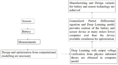
Figure 1. Schematic of the need for physics informed neural network deep learning algorithm in battery technology based sensor devices.

Download: Download full-size image

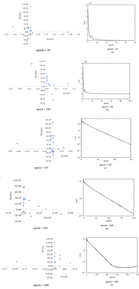
Figure 2. Approach 1 physics informed theory and neural network results for (a) epoch 50, result, loss (b) epoch 100, result, loss (c) epoch 150, result, loss (d) epoch 200, result, loss and (e) epoch 500, result, loss.

Download: Download full-size image

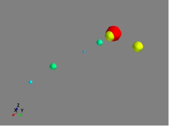
Figure 3. Approach 1 shows the plot in mayavi. The plot is mlab. points3d for 4 variables, charge, frequency, voltage and power. Epoch = 50. The plot shows the color and size of the points to be understood further.

Download: Download full-size image

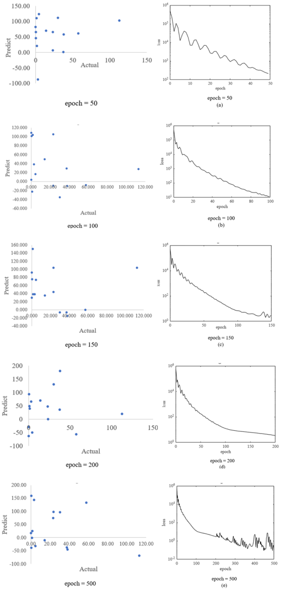
Figure 4. Approach 2 physics informed theory and neural network results for (a) epoch 50, result, loss (b) epoch 100, result, loss (c) epoch 150, result, loss (d) epoch 200, result, loss and (e) epoch 500, result, loss.

The physics informed theory included in the neural network lowers epoch dependency in the accuracy of the predict answers.

Download: Download full-size image

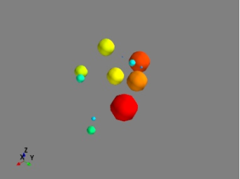
Figure 5. Approach 2 shows the plot in mayavi. The plot is mlab. points3d for 4 variables, charge, frequency, voltage and power. Epoch = 50. The plot shows the color and size of the points to be understood further.

Download: Download full-size image

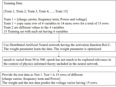
Figure 6. Training of data obtained from physics informed theory approach 2 and neural network algorithm.

Download: Download full-size image

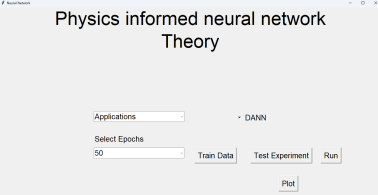
Figure 7. GUI for the Physics informed from theory and neural network.

Download: Download full-size image

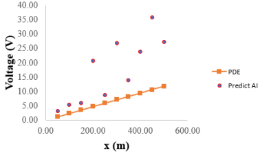
Figure 8. Comparison of physics informed from partial differential equation neural network and the only partial differential equation. In both models we obtain the 1D voltage distribution along the length. Here we use epoch = 50.

5. Conclusions

In this study we develop generalized theory and partial differential equation. We consider battery technology example. We develop physics informed neural network. The physics is included in theory and 1D PDE in the neural network. In our theory we implemented two approaches. The Approach 1 the error is huge. The approach 2 in the physics based from theory included in the neural network the accuracy is 95%. In physics informed from PDE that are included in the neural network the accuracy is 80%. The output voltage is verified with the theory and PDE equations.

Abbreviations

RNN	Recurrent Neural Network
LSTM	Long Short-Term Memory
ReLU	Rectified Linear Unit
ANN	Artificial Neural Network
CNN	Convolutional Neural Network
SVR	Support Vector Regression
DFT	Density Functional Theory
LIB	Lithium Ion Battery
DANN	Distributed Artificial Neural Network
PDE	Partial Differential Equation

Author Contributions

Vishal Venkata Raghavendra Nandigana is the sole author. The author read and approved the final manuscript.

Data Availability Statement

The data is available from the corresponding author upon reasonable request.

Conflicts of Interest

The author declares no conflict of interest.

References

[1]	Raissi, M., Paris, P., George, E. K., Physics-informed neural networks: A deep learning framework for solving forward and inverse problems involving nonlinear partial differential equations, Journal of Computational Physics, 2019, 378, 686-707.
[2]	Norvig, P., Russes S. J., Artificial Intelligence: A Modern Approach, Prentice Hall, 2009.
[3]	Goodfellow, I., Bengio, Y., Courville, A., Deep Learning, MIT Press, 2016.
[4]	Python. Available from: https://www.python.org/ (accessed 8 June 2025).
[5]	Millner, G., Mucke, M., Romaner, L., Scheiber, D., Machine learning mechanical properties of steel sheets from an industrial production route, Materialia, 2023, 30, 101810.
[6]	Rowe, P., Csanyi, G., Alfe, D., Michaelides, A., Development of a machine learning potential for graphene, Phys. Rev. B, 2018, 97, 054303.
[7]	Haghi, S., Hidalgo, M. F. V., Niri, M. F., Daub, R., Marco, J., Machine Learning in Lithium-Ion Battery Cell Production: A Comprehensive Mapping Study, Batteries & Supercaps, 2023, 6, e202300046.
[8]	Gerold, E., Antrekowitsch, H. A Sustainable Approach for the Recovery of Manganese from Spent Lithium-Ion Batteries via Photocatalytic Oxidation. International Journal of Materials Science and Applications. 2022, 11, 66-75.
[9]	D. Roman, S. Saxena, V. Robu, M. Pecht, D. Flynn, Machine learning pipeline for battery state-of-health estimation, Nature Machine Intelligence, 2021, 3, 447-456.
[10]	A. Lanubile, P. Bosoni, G. Pozzato, A. Allam, M. Acquarone, S. Onori, Domain knowledge-guided machine learning framework for state of health estimation in Lithium-ion batteries, Communications Engineering, 2024, 3, 168.
[11]	N. Costa, D. Anseán, M. Dubarry, L. Sanchez, ICFormer: A Deep Learning model for informed lithium-ion battery diagnosis and early knee detection, Journal of Power Sources, Journal of Power Sources, 2024, 592, 233910.
[12]	K. A. Severson , P. M. Attia, et. al. Data-driven prediction of battery cycle life before capacity degradation, Nature Energy, 2019, 4, 383-391.
[13]	Ballard, Z., Brown, C., Madni, A. M., Ozcan, A., Machine learning and computation-enabled intelligent sensor design, Nature Machine Intelligence, 2021, 3, 556-565.
[14]	E. Ozer, J. Kufel, et. al. Malodour classification with low-cost flexible electronics, Nature Communications, 2023, 14, 777.
[15]	T. B. Martin, D. J. Audus, Emerging Trends in Machine Learning: A Polymer Perspective, ACS Polym. Au, 2023, 3, 239-258.
[16]	Forni, T., Baldoni, M., Piane, F. L., Mercuri, F., GrapheNet: a deep learning framework for predicting the physical and electronic properties of nanographenes using images, Scientific Reports, 2024, 14, 24576.
[17]	Dineva, A., Advances in Lithium-Ion Battery Management through Deep Learning Techniques: A Performance Analysis of State-of-Charge Prediction at Various Load Conditions, IEEE 17th International Symposium on Applied Computational Intelligence and Informatics, Romania, 2023, https://ieeexplore.ieee.org/document/10158646
[18]	Payette, J., Vaussenat, F., Cloutier, S., Deep learning framework for sensor array precision and accuracy enhancement, Scientific Reports, 2023, 13, 11237.

Cite This Article

Plain Text BibTeX RIS

APA Style

Nandigana, V. V. R. (2025). Physics Informed Methodology Using Neural Network to Match Measurements in Sensor Devices. Engineering and Applied Sciences, 10(4), 84-95. https://doi.org/10.11648/j.eas.20251004.12

Copy | Download

ACS Style

Nandigana, V. V. R. Physics Informed Methodology Using Neural Network to Match Measurements in Sensor Devices. Eng. Appl. Sci. 2025, 10(4), 84-95. doi: 10.11648/j.eas.20251004.12

Copy | Download

AMA Style

Nandigana VVR. Physics Informed Methodology Using Neural Network to Match Measurements in Sensor Devices. Eng Appl Sci. 2025;10(4):84-95. doi: 10.11648/j.eas.20251004.12

Copy | Download

@article{10.11648/j.eas.20251004.12,
  author = {Vishal Venkata Raghavendra Nandigana},
  title = {Physics Informed Methodology Using Neural Network to Match Measurements in Sensor Devices
},
  journal = {Engineering and Applied Sciences},
  volume = {10},
  number = {4},
  pages = {84-95},
  doi = {10.11648/j.eas.20251004.12},
  url = {https://doi.org/10.11648/j.eas.20251004.12},
  eprint = {https://article.sciencepublishinggroup.com/pdf/10.11648.j.eas.20251004.12},
  abstract = {In this paper we develop physics informed neural network model to solve battery technology. The first model uses physics from the theory. The voltage of the battery is related to the charge carrier, frequency term and power. The theory is used to obtain 15 different voltages. The parameters charge carrier, frequency term, power and voltage are our 15 training data. The training data is trained using Recurrent Neural Network (RNN) Long Short-Term Memory (LSTM). The algorithm determines the weight based on the training data. We study for 50, 100, 150, 200 and 500 epoch. We predict for 15 test cases. The predict file has variables [charge carrier given, frequency given, voltage not given and power given]. We obtain huge error when the training set is given as one file with 15 rows of 4 variables in each row. However the physics from the theory matches with the predict answer for the voltage when the training file has one row of 4 variables that is repeated to study multiple times. We have 15 different training files. We study for 50, 100, 150, 200 and 500 epoch. The dependency on the epoch is visible until 200. The accuracy is 95% for few predict test case results. The predict voltage correlates with the theory. Thus, the model is physics from theory included in the neural network for the first time. Next, we study the physics informed partial differential equation with the neural network. We use 15 training sets. Each training set have 10 rows with variables [grid location, concentration, voltage distribution, frequency term and current]. We use our model to test for one case. The test variables are [same grid location, 1 new concentration, predict the voltage distribution, same frequency term and same current]. We obtain good output matching the actual and the physics. The accuracy is 80%. We study for epoch 50.},
 year = {2025}
}

Copy | Download

TY - JOUR
T1 - Physics Informed Methodology Using Neural Network to Match Measurements in Sensor Devices

AU - Vishal Venkata Raghavendra Nandigana
Y1 - 2025/08/21
PY - 2025
N1 - https://doi.org/10.11648/j.eas.20251004.12
DO - 10.11648/j.eas.20251004.12
T2 - Engineering and Applied Sciences
JF - Engineering and Applied Sciences
JO - Engineering and Applied Sciences
SP - 84
EP - 95
PB - Science Publishing Group
SN - 2575-1468
UR - https://doi.org/10.11648/j.eas.20251004.12
AB - In this paper we develop physics informed neural network model to solve battery technology. The first model uses physics from the theory. The voltage of the battery is related to the charge carrier, frequency term and power. The theory is used to obtain 15 different voltages. The parameters charge carrier, frequency term, power and voltage are our 15 training data. The training data is trained using Recurrent Neural Network (RNN) Long Short-Term Memory (LSTM). The algorithm determines the weight based on the training data. We study for 50, 100, 150, 200 and 500 epoch. We predict for 15 test cases. The predict file has variables [charge carrier given, frequency given, voltage not given and power given]. We obtain huge error when the training set is given as one file with 15 rows of 4 variables in each row. However the physics from the theory matches with the predict answer for the voltage when the training file has one row of 4 variables that is repeated to study multiple times. We have 15 different training files. We study for 50, 100, 150, 200 and 500 epoch. The dependency on the epoch is visible until 200. The accuracy is 95% for few predict test case results. The predict voltage correlates with the theory. Thus, the model is physics from theory included in the neural network for the first time. Next, we study the physics informed partial differential equation with the neural network. We use 15 training sets. Each training set have 10 rows with variables [grid location, concentration, voltage distribution, frequency term and current]. We use our model to test for one case. The test variables are [same grid location, 1 new concentration, predict the voltage distribution, same frequency term and same current]. We obtain good output matching the actual and the physics. The accuracy is 80%. We study for epoch 50.
VL - 10
IS - 4
ER -

Copy | Download

Author Information

Vishal Venkata Raghavendra Nandigana

206 Fluid Systems Laboratory, Department of Mechanical Engineering, Indian Institute of Technology Madras, Chennai, India

Biography: Vishal Venkata Raghavendra Nandigana is Associate Professor in Department of Mechanical Engineering in Indian Institute of Technology Madras, Chennai, India

Research Fields: micro-nanofluidic integrated systems, artificial intelligence, polymers, membranes

Contact Email

http://orcid.org/0009-0000-6260-6567

Download PDF

Submit an Article

Table 1

Table 1. The 15 training set are given. Each row has 4 variables. The variables are charge carrier, frequency term, voltage and power. Variables to calculate the voltage. We provide in one file.
Table 2

Table 2. Test parameters of 15. We have to predict the voltage for the given variables. We have to use approach 1 and approach 2 to provide the predicted voltage.
Table 3

Table 3. Parameters with 5 columns. Column 1 has finite grid points, column 2 has the concentration, column 3 has voltage corresponding to each grid point, column 4 has frequency and column 5 has current. Parameters with 5 columns. Column 1 has finite grid points, column 2 has the concentration, column 3 has voltage corresponding to each grid point, column 4 has frequency and column 5 has current.

Plain Text BibTeX RIS

APA Style

Nandigana, V. V. R. (2025). Physics Informed Methodology Using Neural Network to Match Measurements in Sensor Devices. Engineering and Applied Sciences, 10(4), 84-95. https://doi.org/10.11648/j.eas.20251004.12

Copy | Download

ACS Style

Nandigana, V. V. R. Physics Informed Methodology Using Neural Network to Match Measurements in Sensor Devices. Eng. Appl. Sci. 2025, 10(4), 84-95. doi: 10.11648/j.eas.20251004.12

Copy | Download

AMA Style

Nandigana VVR. Physics Informed Methodology Using Neural Network to Match Measurements in Sensor Devices. Eng Appl Sci. 2025;10(4):84-95. doi: 10.11648/j.eas.20251004.12

Copy | Download

@article{10.11648/j.eas.20251004.12,
  author = {Vishal Venkata Raghavendra Nandigana},
  title = {Physics Informed Methodology Using Neural Network to Match Measurements in Sensor Devices
},
  journal = {Engineering and Applied Sciences},
  volume = {10},
  number = {4},
  pages = {84-95},
  doi = {10.11648/j.eas.20251004.12},
  url = {https://doi.org/10.11648/j.eas.20251004.12},
  eprint = {https://article.sciencepublishinggroup.com/pdf/10.11648.j.eas.20251004.12},
  abstract = {In this paper we develop physics informed neural network model to solve battery technology. The first model uses physics from the theory. The voltage of the battery is related to the charge carrier, frequency term and power. The theory is used to obtain 15 different voltages. The parameters charge carrier, frequency term, power and voltage are our 15 training data. The training data is trained using Recurrent Neural Network (RNN) Long Short-Term Memory (LSTM). The algorithm determines the weight based on the training data. We study for 50, 100, 150, 200 and 500 epoch. We predict for 15 test cases. The predict file has variables [charge carrier given, frequency given, voltage not given and power given]. We obtain huge error when the training set is given as one file with 15 rows of 4 variables in each row. However the physics from the theory matches with the predict answer for the voltage when the training file has one row of 4 variables that is repeated to study multiple times. We have 15 different training files. We study for 50, 100, 150, 200 and 500 epoch. The dependency on the epoch is visible until 200. The accuracy is 95% for few predict test case results. The predict voltage correlates with the theory. Thus, the model is physics from theory included in the neural network for the first time. Next, we study the physics informed partial differential equation with the neural network. We use 15 training sets. Each training set have 10 rows with variables [grid location, concentration, voltage distribution, frequency term and current]. We use our model to test for one case. The test variables are [same grid location, 1 new concentration, predict the voltage distribution, same frequency term and same current]. We obtain good output matching the actual and the physics. The accuracy is 80%. We study for epoch 50.},
 year = {2025}
}

Copy | Download

TY - JOUR
T1 - Physics Informed Methodology Using Neural Network to Match Measurements in Sensor Devices

Copy | Download