1. Introduction
The global health and fitness landscape is increasingly shaped by data-driven technologies, creating a demand for personalized health metrics. A cornerstone of this personalization is the accurate estimation of energy expenditure, quantified as calories burned. This metric is vital for individuals managing weight, optimizing athletic performance, or achieving specific fitness goals
| [1] | Zeng, N., Amin, Z., Pope, Z. C., & Gao, Z. (2026). Wearable Devices in Promoting Physical Activity and Health. In Physical Activity, Health and Emerging Technologies (pp. 89-114). Routledge. |
[1]
. Energy expenditure is the total amount of energy used by the human body to maintain physiological functions and perform physical activities. According to energy balance theory, total energy expenditure consists of three major components: Basal Metabolic Rate (BMR), Thermic Effect of Food (TEF) and Activity Energy Expenditure (AEE). Of all this, the Activity Energy Expenditure is the most variable component and represents energy used during physical movement and exercise. It is influenced by several factors, including heart rate, body weight, age, physical fitness, activity intensity, and activity duration
| [2] | Kiedrowski, M. (2024). Assessment of energy balance in nutritional counseling–fact or myth?. Advances in Hygiene and Experimental Medicine= Postepy Higieny i Medycyny Doswiadczalnej, 78(1), 82-87. |
[2]
. Traditional calorie estimation methods rely on generalized formulas and metabolic equivalent task (MET) values. However, these methods assume uniform energy expenditure across individuals and fail to account for individual physiological differences such as body composition, metabolic efficiency, and genetic factors
| [2] | Kiedrowski, M. (2024). Assessment of energy balance in nutritional counseling–fact or myth?. Advances in Hygiene and Experimental Medicine= Postepy Higieny i Medycyny Doswiadczalnej, 78(1), 82-87. |
[2]
. Research has shown that energy expenditure varies significantly among individuals performing identical activities due to variations in metabolism, cardiovascular efficiency, and muscle mass. This limitation highlights the need for intelligent systems capable of learning individual physiological patterns and accurately predicting calorie expenditure using data-driven approaches such as machine learning. Machine Learning (ML), a transformative subset of Artificial Intelligence, offers a powerful solution. Unlike static formulas, ML models can learn complex, non-linear relationships from high-dimensional datasets. By training on diverse features, such as anthropometric data (age, weight, height, and gender) and dynamic physiological signals (heart rate and activity type), an ML model can deliver highly personalized and accurate predictions of caloric burn
| [3] | Ansari, M. A., Jayaswal, R., Singh, D. K., & Singh, N. (2026). Nutrition Meets Al: Opportunities in Recommender. Advancing Equity in Global Healthcare Systems, 401. |
[3]
. In related development,
| [4] | LeCun, Y., Bengio, Y., & Hinton, G. (2015). Deep learning. nature, 521(7553), 436-444. |
[4]
demonstrated that deep learning, a subset of Machine learning outperforms the traditional machine learning models in tasks involving complex data and hence more suitable for predicting calories burned due the complex nature of its dataset. Deep learning models in particular Neural network model are known as universal function approximations capable of approximating any nonlinear function with sufficient training data
| [5] | Haykin, S. (2009). Neural networks and learning machines, 3/E. Pearson education india. |
[5]
which makes them suitable for regression problems involving physiological prediction. Calorie prediction is a regression problem because the output variable (calories burnt) is continuous. Neural network models such as ANN, DNN, and RNN can be trained using supervised learning to predict calorie expenditure accurately as supervised learning enables neural networks to learn patterns from physiological data and improve prediction accuracy over time. Although several researches has been carried out in the field of calories expenditures however, most of the existing systems using conventional formulas and wearable algorithms are not personalized
| [6] | Elfouly, T., & Alouani, A. (2025). A comprehensive survey on wearable computing for mental and physical health monitoring. Electronics, 14(17), 3443. |
[6]
while most existing machine learning models for calories expenditure lack adequate data utilization and adaptability
| [7] | Smith, K. J., Endsley, T. C., & Clark, T. K. (2026). Predicting situation awareness from physiological signals. IEEE Transactions on Human-Machine Systems. |
[7]
. This work is designed to directly address these problems by developing and optimizing neural network regression models (ANN, DNN, RNN) for predicting calories burned. It is an intelligent, data-adaptive system that provides a personalized and reliable real time calorie prediction tool by leveraging computational intelligence thereby providing scientifically grounded support for human fitness endeavors. The motivation for comparing these neural network models leys with their similarities and difference as Artificial Neural Networks can learn relationships between physiological inputs such as heart rate, weight, age, and activity duration, and energy expenditure for personalized predictions. Deep Neural Networks can learn deeper feature representations from data to automatically identify important patterns in physiological data while Recurrent Neural Networks are particularly effective because they can analyze time-series physiological data such as continuous heart rate measurements. By implementing and comparing multiple neural network architectures within a complete system, this paper contributes to improving the accuracy and practical applicability of calorie prediction systems. The outcome of this work is a functional neural network–based calorie prediction system capable of providing accurate, reliable, and personalized calorie expenditure estimates in real time.
2. Related Works
Neural networks have become one of the most effective tools for predicting calories burnt due to their ability to model complex nonlinear relationships between physiological variables and energy expenditure. The application of neural networks in predicting energy expenditure has been widely studied and several researchers have proposed neural network–based approaches to improve the accuracy of calorie prediction systems. To illustrate thus fact,
| [8] | Zhu, J., Pande, A., Mohapatra, P., & Han, J. J. (2015, October). Using deep learning for energy expenditure estimation with wearable sensors. In 2015 17th International Conference on E-health Networking, Application & Services (HealthCom) (pp. 501-506). IEEE. |
[8]
developed a neural network model using wearable physiological sensors data to estimate energy expenditure. Their study demonstrated that neural networks could effectively learn complex relationships between physiological signals and calorie expenditure, providing more accurate predictions compared to traditional estimation methods. In the same Vein,
| [4] | LeCun, Y., Bengio, Y., & Hinton, G. (2015). Deep learning. nature, 521(7553), 436-444. |
[4]
established the theoretical foundation of deep learning and demonstrated that deep neural networks can learn hierarchical representations from data and achieve superior performance in prediction tasks. Their research confirmed that deep learning models are highly effective for complex prediction problems involving nonlinear relationships. Equally,
| [9] | Tao, L., Burghardt, T., Mirmehdi, M., Damen, D., Cooper, A., Hannuna, S.,... & Craddock, I. (2016, November). Calorie counter: RGB-depth visual estimation of energy expenditure at home. In Asian Conference on Computer Vision (pp. 239-251). Cham: Springer International Publishing. |
[9]
developed a vision-based calorie prediction system using neural networks and RGB-D sensor data. Their system successfully estimated calorie expenditure in real-life environments and demonstrated that neural network models could accurately predict energy expenditure using sensor-based physiological and motion data.
Deep learning and recurrent neural networks are particularly effective for time-series prediction tasks, making them suitable for modeling sequential physiological data such as heart rate signals
| [10] | Goodfellow, I., Bengio, Y., Courville, A., & Bengio, Y. (2016). Deep learning (Vol. 1, No. 2, pp. 1-800). Cambridge: MIT press. |
[10]
. The study in
| [11] | Masullo, A., Burghardt, T., Damen, D., Hannuna, S., Ponce-López, V., & Mirmehdi, M. (2018). CaloriNet: From silhouettes to calorie estimation in private environments. arXiv preprint arXiv: 1806.08152. |
[11]
, proposed CaloriNet, a deep neural network architecture designed to estimate calorie expenditure using accelerometer data and temporal motion signals. Their model combined convolutional neural networks and temporal modeling techniques to improve accuracy. The results demonstrated that neural network–based models outperformed traditional calorie estimation methods, highlighting the importance of deep learning in energy expenditure prediction. Similarly,
| [12] | Chen, K., Zhang, D., Yao, L., Guo, B., Yu, Z., & Liu, Y. (2021). Deep learning for sensor-based human activity recognition: Overview, challenges, and opportunities. ACM Computing Surveys (CSUR), 54(4), 1-40. |
[12]
developed a deep learning model that used wearable sensor data such as accelerometer and heart rate measurements to estimate energy expenditure. Their study demonstrated that neural networks could effectively learn relationships between physiological variables and calorie expenditure. The model showed improved prediction accuracy compared to traditional regression models, confirming the effectiveness of neural networks in physiological prediction tasks. In related development,
| [13] | Lopes, J. M., Figueiredo, J., Fonseca, P., Cerqueira, J. J., Vilas-Boas, J. P., & Santos, C. P. (2022). Deep learning-based energy expenditure estimation in assisted and non-assisted gait using inertial, EMG, and heart rate wearable sensors. Sensors, 22(20), 7913. Masullo, A., et al. (2018). CaloriNet: From silhouettes to calorie estimation in private environments. |
[13]
proposed a deep learning–based system using wearable sensors, including inertial sensors, electromyography (EMG), and heart rate monitors, to estimate energy expenditure. Their research evaluated deep neural network models such as Long Short-Term Memory (LSTM), a type of recurrent neural network, and convolutional neural networks (CNN). The results showed that deep learning models could accurately estimate energy expenditure and provide real-time predictions, offering a practical alternative to indirect calorimetric, which is invasive and unsuitable for continuous monitoring. Also,
| [14] | Lee, C. J., & Lee, J. K. (2024). IMU-based energy expenditure estimation for various walking conditions using a hybrid CNN–LSTM model. Sensors, 24(2), 414. |
[14]
developed a hybrid CNN–LSTM neural network model to estimate energy expenditure using wearable inertial measurement unit (IMU) sensors. Their study demonstrated that combining convolutional neural networks and recurrent neural networks significantly improved prediction accuracy. The CNN component extracted spatial features from sensor data, while the LSTM component captured temporal dependencies. This hybrid approach demonstrated superior performance compared to traditional machine learning methods. Furthermore,
| [15] | Babakhani, S., Remy, D., & Roitberg, A. (2025). Deep learning for metabolic rate estimation. arXiv. Dataset used: Multimodal bio signals including heart rate, respiration, accelerometry, EMG, with grouped sensor inputs.
https://arxiv.org/abs/2511.09276 |
[15]
conducted a comparative study of neural network architectures for energy expenditure prediction using bio signals such as heart rate, respiration, and accelerometer data. Their results showed that neural network models achieved significantly lower prediction errors compared to classical regression models. The study also emphasized the importance of adaptive modeling to account for individual physiological differences. Despite these advancements, several gaps still exist in the current body of research. Most existing calorie prediction systems lack personalization capabilities. They often rely on generalized models trained on population-level data rather than models that can adapt to individual users. Many existing studies also focused primarily on developing and evaluating neural network models in controlled research environments without implementing complete systems that can be used in real-world applications. In many cases, the models are tested using pre-existing datasets rather than integrated into functional systems capable of collecting input data, processing it, and providing real-time predictions to users. There is therefore, a need for practical systems that compare the efficiencies of different neural network models under the same research condition and integrate the best neural network model into functional calorie burned prediction applications.
3. Research Methodology
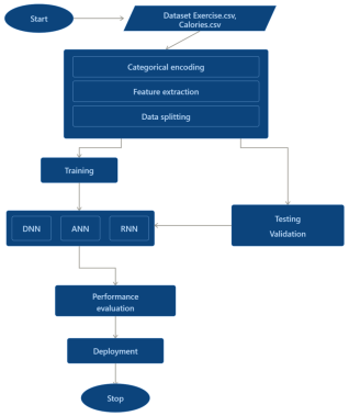
The research methodology adopted in this study involves description of dataset, data preprocessing pipeline, feature engineering strategy, neural network architectures employed for the Artificial Neural Network (ANN), Deep Neural Network (DNN), and Recurrent Neural Network proxy (RNN) as well as model evaluation and deployment. The methodology follows a structured, reproducible machine learning pipeline consistent with quantitative research methodology. The proposed methodology for this study is presented in
Figure 1.
Figure 1. Proposed Research Methodology.
3.1. Dataset Description
Two datasets are acquired from the Kaggle Machine Learning Repository. These two datasets are Exercise.csv, which contains demographic and exercise session attribute values, and Calories.csv, which contains the corresponding calorie expenditure values. These two datasets are joined on the User_ID column using an inner join to form a single dataset containing 15,000 data points and 9 variables (prior to feature engineering).
Table 1 provides a summary of the dataset attributes.
Table 1. Summary of Raw Dataset Features.
Feature | Type | Description | Range |
User_ID | Integer | Unique participant identifier | 10,001,159 – 19,999,647 |
Gender | Categorical | Biological sex of participant | male (7,447), female (7,553) |
Age | Integer | Age in years | 20 – 79 |
Height | Integer | Height in centimetres | 123 – 222 |
Weight | Integer | Body weight in kilograms | 36 – 132 |
Duration | Integer | Exercise duration in minutes | 1 – 30 |
Heart_Rate | Integer | Average heart rate during exercise (bpm) | 67 – 128 |
Body_Temp | Float | Body temperature during exercise (°C) | 37.1 – 41.5 |
Calories | Float | Target: Calories burnt (kcal) | 1.0 – 314.0 |
3.2. Dataset Preprocessing
The unified dataset undergoes series of preprocessing steps to ensure proper cleaning and makes it ready for training the neural network models. The first step of preprocessing is categorical encoding, where the gender variable is encoded using binary encoding into a numeric variable, i.e., male=1 and female=0, so that it is suitable for neural network models training. The second step of preprocessing is feature engineering, where 11 features were created from existing features such as Body Mass Index (BMI), Body Surface Area (BSA), HR_Duration, Metabolic_Load, among others, increasing the total number of features from 9 to 18. The third step of preprocessing was feature standardization which was performed using z-score normalization, defined as:
Where is the original feature value, is the mean of the feature, and is the standard deviation. This transformation rescales all features to have a mean of 0 and a standard deviation of 1, which improves convergence speed and stability for many machine learning algorithms. The fourth step of preprocessing was data splitting, where the dataset is divided into a training set containing 75% of the data (11,250 samples) and a test set containing 25% of the data (3,750 samples).
3.3. Neural Network Model Development
This study employs three neural network architectures ANN, DNN, and a Recurrent Neural Network proxy (RNN_proxy) to model the complex, non-linear relationship between physiological features and calorie expenditure. All three models are based on the Multi-Layer Perceptron (MLP) framework and operate as feed forward neural networks trained using back propagation and gradient-based optimization. The ANN is a relatively shallow architecture consisting of two hidden layers with 256 and 128 neurons, respectively. The ANN receives an input vector of 18 features and propagates this information through successive linear transformations followed by non-linear activation functions. At each layer, the computation is defined as:
Where is the output of layer represents the weight matrix, is the bias vector, and is the activation function. In this study, the Rectified Linear Unit (ReLU) is used, defined as:
The ANN’s shallow depth allows it to efficiently learn general patterns in the data while maintaining low computational complexity. However, its limited number of layers restricts its ability to capture deeper hierarchical relationships among features. The Deep Neural Network (DNN) extends the ANN by introducing four hidden layers with progressively decreasing neuron sizes (256, 128, 64, 32). This architecture enables hierarchical feature learning; where early layers capture simple patterns and deeper layers combine these into more abstract representations. The forward propagation process remains the same as in the ANN but is applied across more layers, allowing deeper abstraction. The final output of the network is computed as:
Where L denotes the output layer. The progressive reduction in dimensionality (from 256 to 32 neurons) acts as an information bottleneck, forcing the network to retain only the most relevant features. This improves generalization and reduces redundancy, making the DNN very effective in capturing complex non-linear relationships and typically yielding good predictive accuracy. The Recurrent Neural Network proxy (RNN_proxy) is designed as a wide architecture with three hidden layers (256, 256, 128) to increasing representational capacity through its wider layers. The dual 256-neuron hidden layers create a high-dimensional feature space capable of modeling intricate interactions among input variables. The computations follow the same feed forward structure as ANN and DNN. Recurrent neural network operates using temporal dependencies defined as:
(5)
Where h_t represents the hidden state at time step t, and h_(t−1) is the previous hidden state.
All three models are trained using the back propagation algorithm, where the objective is to minimize a loss function, typically the Mean Squared Error (MSE), defined as:
Where is the actual value and is the predicted value. The optimisation process iteratively updates model weights using gradient descent-based methods: Adam optimiser. During training, gradients of the loss function with respect to the weights are computed and used to adjust parameters in the direction that minimizes prediction error. Google Colab was utilized for training models and conducting experiments to leverage the capabilities of GPU acceleration, which significantly reduced the training time for the neural network models. The implementation of the machine learning models was done with the help of the Tensor Flow library, which was used as the primary framework for the development of the ANN, DNN, and RNN models. The Keras library, which is a high-level application programming interface (API), was used for the development of the neural network models due to its simplicity and modularity, as it is a part of the Tensor Flow framework. Other libraries were also used to support the development process. The Scikit-learn library was used for data preprocessing feature scaling, and the computation of the performance of the models. The Pandas and NumPy libraries were used for data manipulation and numerical computation. Additionally, the Matplotlib and Seaborn libraries were used for data visualization.
3.4. Model Evaluation Metrics
The predictive performance of the developed models was evaluated using nine complementary evaluation metrics: R2, Adjusted R2, RMSE, MAE, MedAE, MAPE, EVS, Pearson correlation coefficient, and Maximum Error. These metrics collectively assess goodness of fit, average error magnitude, robustness to outliers, correlation strength, and worst-case prediction behavior. Coefficient of Determination (R2) measures the proportion of variance in the dependent variable explained by the model. It provides a global indication of model fit where values close to 1 indicates that the model explains almost all variability in the data, while values close to 0 indicates poor explanatory power. However, R2 alone does not account for model complexity. It is given by the relation:
(7)
Where actual value, = predicted value, = mean of actual values, = number of observations. Adjusted R2 improves upon R2 by incorporating a penalty for the number of predictors. This prevents artificially high scores when irrelevant features are added. It is particularly useful in this study due to the inclusion of engineered features, ensuring that improvements in performance are meaningful and not due to overfitting.
(8)
Where is the number of predictors and is the number of observations. Root Mean Squared Error (RMSE) measures the standard deviation of prediction errors. Because errors are squared before averaging, larger errors have a disproportionately high impact. This makes RMSE highly sensitive to outliers and useful for identifying models that produce large deviations from actual values.
Mean Absolute Error (MAE) computes the average magnitude of errors without squaring them, making it more interpretable and less sensitive to extreme values than RMSE. It provides a clear indication of the typical prediction error in the same units as the target variable (kcal).
Median Absolute Error (MedAE) represents the median of absolute errors and is highly robust to outliers. Unlike MAE and RMSE, it is not influenced by extreme prediction errors, making it a reliable measure of the model’s typical performance under normal conditions.
(11)
Mean Absolute Percentage Error (MAPE) expresses prediction errors as percentages, enabling scale-independent evaluation. This is particularly useful when comparing performance across datasets or models. Lower MAPE values indicate higher predictive accuracy, with values below 10% generally considered highly accurate.
(12)
Explained Variance Score (EVS) measures the proportion of variance in the target variable captured by the model’s predictions. Unlike R2, EVS does not penalize systematic bias (consistent over- or under-prediction). It focuses purely on how well the variability in the data is reproduced.
(13)
Pearson Correlation Coefficient (r) measures the strength and direction of the linear relationship between actual and predicted values. Values range from −1 to 1. A value close to 1 indicates a strong positive linear relationship, meaning predictions closely follow the trend of actual values.
(14)
Where is the mean of predicted values?
Maximum Error (MaxError) captures the largest single prediction error made by the model. It is critical for evaluating model reliability, especially in applications where large prediction failures are unacceptable. These metric highlights worst-case behavior rather than average performance.
(15)
3.5. System Prototype Development
Lastly, the best-performing model is chosen for the deployment of the system. The system is built using the Flask framework and Visual Studio Code. It is a web-based system that allows the user to input physiological and exercise-related parameters. It provides real-time predictions of calorie expenditure. It also provides the user with other health-related benefits like BMI, metabolic load, and exercise intensity level.
4. Results and Discussion
This section includes Exploratory Data Analysis (EDA) of the dataset and evaluation result of the proposed models based on criteria: R2, Root Mean Squared Error (RMSE), Mean Absolute Error (MAE), and Mean Absolute Percentage Error (MAPE).
4.1. Exploratory Data Analysis (EDA)
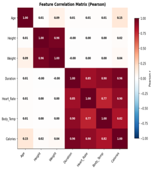
The correlation matrix (Pearson) from
Figure 2 provides a clear quantitative overview of the linear relationships among the features and the target variable (Calories). The most striking observation is the very strong positive correlation between Duration and Calories (r ≈ 0.96), indicating that exercise duration is the single most influential predictor of calorie expenditure. Similarly, Heart Rate (r ≈ 0.90) and Body Temperature (r ≈ 0.82) also show strong positive correlations with Calories, reflecting the physiological reality that increased cardiovascular activity and thermoregulation are associated with higher energy expenditure. In contrast, Age (r ≈ 0.15), Height (r ≈ 0.02), and Weight (r ≈ 0.04) exhibit weak correlations with Calories, suggesting that demographic and static body measurements alone are poor predictors without interaction with activity-related variables. Additionally, a notable multi-collinearity exists between Height and Weight (r ≈ 0.96), indicating strong linear dependence, which justifies the introduction of derived features such as BMI during feature engineering. Overall, the correlation structure validates the importance of dynamic physiological features over static attributes.
Figure 2. Correlation Matrix Plot.
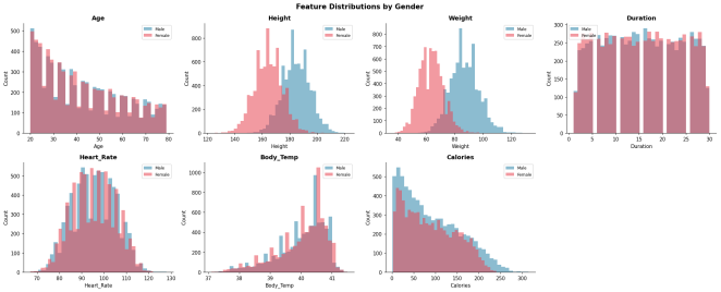
The feature distribution plots by gender reveal important insights into the dataset’s structure and balance. The Age distribution appears approximately uniform across the range of 20 to 79 years, with male and female distributions nearly overlapping, confirming no age-related sampling bias. Height and Weight distributions show clear separation between genders, with males generally taller and heavier than females, which are consistent with biological expectations. However, despite these differences, their weak correlation with Calories suggests that their effect is indirect. The Duration distribution is nearly uniform across the range of 1 to 30 minutes for both genders, ensuring that the dataset captures a wide variety of exercise intensities. Heart Rate follows an approximately normal distribution centered on mid-range values (≈95 bpm), while Body Temperature is slightly left-skewed and tightly concentrated between 39°C and 41.5°C, indicating limited variability. The Calories distribution is right-skewed, with a high concentration of lower values and a long tail extending toward higher calorie burns. Importantly, male and female calorie distributions overlap significantly, suggesting that gender alone does not strongly differentiate calorie expenditure when other features are considered.
Figure 3. Feature Distribution.
The scatter plots of key features from
Figure 3 against Calories further reinforce the findings from the correlation analysis while revealing the nature of relationships beyond simple linearity. The Duration vs Calories plot shows a near-perfect linear relationship, with data points tightly clustered along the regression line, confirming Duration as the dominant predictor. The Heart Rate vs Calories plot also demonstrates a strong positive relationship, though with slightly more dispersion, indicating that heart rate contributes significantly but with some variability. The Body Temperature vs Calories relationship appears non-linear, exhibiting a curved upward trend, suggesting that small increases in temperature at higher levels correspond to disproportionately larger calorie burns. In contrast, the Weight vs Calories plot shows a weak and diffuse relationship, with a broad spread of calorie values across all weight ranges, confirming its limited standalone predictive power. Similarly, the Age vs Calories plot displays a very weak trend with high variance, indicating that age has minimal direct influence on calorie expenditure.
Figure 4. Key Scattered Plots.
Across all scatter plots, the regression lines (OLS fit) highlight the general trend, while the dispersion of points indicates the variability captured by the models. The color-coding by gender shows substantial overlap in all relationships, reinforcing that physiological and activity-based variables dominate prediction performance over demographic factors. This EDA demonstrates that calorie expenditure is primarily driven by exercise intensity and duration-related features, while demographic variables play a secondary role. The strong correlations and clear patterns observed justify the feature engineering approach and support the use of neural networks as non-linear model capable of capturing these complex interactions.
4.2. Model Results
The results from
Table 2 show that all three neural network models ANN, DNN, and RNN performed exceptionally well, with very high R
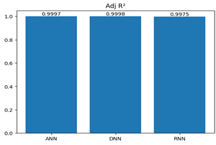
2 values (≥ 0.9975). This indicates that each model explains over 99% of the variance in calorie expenditure, demonstrating strong predictive capability as seen in
Figure 5.
Table 2. Result Presentation.
Model | R2 | Adj R2 | RMSE | MAE | MedAE | MAPE (%) | EVS | Pearson r | Max Error |
ANN | 0.9997 | 0.9997 | 1.011 | 0.734 | 0.554 | 2.66% | 0.9997 | 0.9999 | 10.16 |
DNN | 0.9998 | 0.9998 | 0.889 | 0.656 | 0.530 | 1.88% | 0.9998 | 0.9999 | 11.93 |
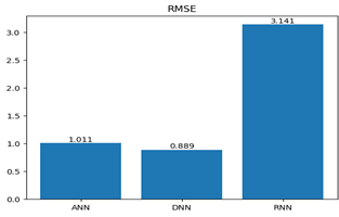
RNN | 0.9975 | 0.9975 | 3.141 | 0.746 | 0.420 | 1.47% | 0.9975 | 0.9988 | 84.23 |
Figure 5. Adjusted R2 Scores.
Figure 6. Mean Absolute Error Scores.
The ANN resulted in a high R2 of 0.9997, with low error rates as well (RMSE of 1.011, MAE of 0.734). This shows the effectiveness of the shallow neural network. However, the higher MAPE of 2.66% shows a slightly higher relative error compared to the other models. The DNN surpassed the performance of the ANN, with a higher R2 of 0.9998, lower error rates of 0.889 (RMSE) and 0.656 (MAE), respectively, proving the effectiveness of the deeper model on the calorie expenditure data. Moreover, the lower MAPE of 1.88% shows the higher accuracy of the model. Thus, the DNN proves to be the best standalone model.
The RNN model had the lowest R
2 value (0.9975) and the highest RMSE (3.141), which signifies a relatively poor performance. Though the MAPE of the RNN model (1.47%) is relatively very low, the high maximum error (84.23) may be attributed to the fact that the RNN model is suitable for sequential data, but the prediction of calorie expenditure does not seem to be dependent on time series. The comparative analysis of the neural network model Mean Absolute Error Score is shown in
Figure 6. In general, the most reliable model among the neural networks is the DNN model because of its high accuracy and low error rate. The ANN model is also good but slightly underperforms compared to the DNN model because of its limited depth. The RNN model is less suitable for this task because of the lack of strong patterns.
4.3. Analysis of Model Convergence
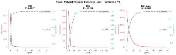
Figure 7 presents the training dynamics of the ANN, DNN, and RNN, showing the variation of training loss and validation R
2 across epochs. These curves illustrate the learning efficiency, convergence speed, and generalization ability of each model.
Figure 7. Analysis of Model Convergence.
From the graph of the ANN model, it is evident that the model converges very rapidly. The training loss is declining rapidly to almost zero within the first little iteration (approximately 3-5). At the same time, the R2 value is increasing rapidly to almost 0.9997 and then becomes stable. Therefore, it can be concluded that the model is learning the major patterns of the dataset. However, the extremely rapid convergence of the model implies that it is not able to efficiently learn complex patterns. From the graph of the DNN model, it is evident that the model is converging optimally. The training loss is declining rapidly to almost zero. However, the rate of decline is slightly lower compared to that of the ANN model. At the same time, the R2 value is increasing to almost 0.9998 and then becomes stable. The R2 value is stable without any fluctuations. Therefore, it can be concluded that the model is learning complex patterns optimally. On the other hand, the RNN shows a slower and less efficient convergence behavior. The loss decreases gradually over a longer number of epochs, up to 120, while the R2 of the validation data stabilizes at a lower level, approximately 0.9975. It can be noticed that the learning efficiency of the model is reduced. The slower convergence, as well as the slight irregularities, shows the difficulties of the model in learning the data. These difficulties are justified, as the RNN model is more appropriate for sequential data, while the data used in the present study is non-sequential. In conclusion, all models show efficient convergence, as indicated by the continuously decreasing loss and the increasing R2. However, the best convergence behavior is recorded from the DNN model, which shows stability, accuracy, and efficiency during learning. The ANN model shows good convergence behavior, although with lower precision, while the RNN model is less efficient, as indicated by the slower learning behavior.
4.4. Deployment
Figure 8 shows the deployed calorie expenditure prediction system that offers an interactive user interface to compute the calories expended according to the specific inputs provided. The system includes the integration of the trained models developed through the machine learning techniques ANN, DNN, and RNN into a system that can function to make predictions in real-time. The interactive interface is divided into two main areas: the input section on the left where users can input their information and other parameters related to their workout routines, and the output section on the right where users can see the predictions made. The system allows users to make their choice of model to use in the predictions; however, it is recommended that the Deep Neural Network (DNN) model is used to make the predictions since it is the best. Once the required information is entered into the system, it can then make the predictions and display the calories expended as well as other health-related information such as Body Mass Index (BMI), metabolism load, and intensity of workout. The system is created using the Flask API.
Figure 8. Calories Model Deployment Using Flask.
The model uses various physiological and activity-based input variables: Gender, Age, Height and weight, BMI, Duration, Heart rate, and Body temperature to make predictions and generate all necessary outputs. The developed system has proven to be effective in transforming machine learning models into an application that can be used to predict calories in real-time, thus being instrumental in ensuring health insights, which can be very beneficial to an individual.





 Share This Article
 Twitter
 Linked In
 Facebook



 Copy
 Download