Research Article | | Peer-Reviewed

On the Unreasonable Weak Effectiveness in Overlapping the Turbulent Flow Theoretical Models and the Prediction Models of Extreme Weather Events

Received: 25 May 2025     Accepted: 11 June 2025     Published: 14 July 2025
Views:       Downloads:
Abstract

We try to understand the difficulties in using both theoretical modelling of turbulence and the theoretical essentialization of extreme climate events for the practical prediction calculations of the climate phenomena. We conceptually understand what contributes to rapid intensification of natural phenomena like heatwaves, floods, tornadoes or hurricanes. Predicting their rapid intensification is a completely different matter. This paper is devoted to the sudden and not frequent occurrence of extremely violent events that appear randomly in space and time in which turbulence is generally the main physical support. Coherence and regularities in this case are not yet clearly delineated. A close analogy between the theory of turbulence and the quantum theory of fields seems to me very attractive. On one hand we do have a rough, practical, working understanding of many turbulence phenomena but certainly far from a theory capable of describing them completely. On the other hand, there are hardwired patterns in nature (the well known tornado funnel pattern, for instance) and also systematic perturbations, induced by factors external to the local weather system. Under a critical combination of initial conditions and interactions an extreme event is triggered. Theoretical models available in physics, injected in the study of extreme climate phenomena could be of great use in resolving the immediacy to the consequences of global warming. We are compelled to adjust to wildly unpredictable circumstances and radical uncertainty. We try to achieve a better understanding of why the respective fields of climate (extreme events) models and theoretical mathematical models of turbulence physics are not sufficiently if not even essentially overlapping as they should be normally.

Published in American Journal of Modern Physics (Volume 14, Issue 4)
DOI 10.11648/j.ajmp.20251404.11
Page(s) 167-185
Creative Commons

This is an Open Access article, distributed under the terms of the Creative Commons Attribution 4.0 International License (http://creativecommons.org/licenses/by/4.0/), which permits unrestricted use, distribution and reproduction in any medium or format, provided the original work is properly cited.

Copyright

Copyright © The Author(s), 2025. Published by Science Publishing Group

Keywords

Turbulence, Extreme Climate Events, Mathematical Theoretical Modelling, Statistical Predictive Models, Overlapping Models

1. Introduction
The consequences of global warming show two fundamental features: 1) slowly varying and constant evolution of climate changes and 2) sudden and not frequent occurrence of extremely violent events that appear randomly in space and time. The climate balance is very sensitive to changing conditions, local and regional. The climate system is coherent (in the sense that there exists a definite phase relationship between different states of the system) and it is also clearly unpredictable, full of many dramatic events. In 1) the slow evolution often hides the unpredictable occurrence of critical thresholds related to global warming or other anthropogenic factors like pollution. In the meantime such changes could trigger a series of ecological chain reactions. In 2) turbulence plays an essential role inducing a character of pure unpredictability; such flows enhance transport of heat, humidity and momentum. Sometimes this enhancement is the evidence that a flow is turbulent. Turbulence involves many different length-scales and frequencies, from the inertial range of the large-scale eddies to the viscous range of the small-scale ones, and the various quantities of the flow (speed, momentum, vorticity, heat, pressure, etc.) show a random variation, i.e. irregular and disordered behavior. Even a very weak perturbation introduced in the turbulent system may completely change its behavior. The flow is then unstable and unpredictable. In consequence, a detailed description of every possible state of equilibrium is not possible. Nevertheless, there is experimental evidence that many turbulent flows have strongly coherent, quite predictable structures . Turbulent flows have both organized and apparently disorganized parts. The more or less organized turbulence forms (due to a kind of instability of the flow) coherent or organized structures describing spatial patterns. We have to find a way to model theoretically a turbulent flow, mathematically and/or numerically, “to produce a smooth flow where high frequencies have been filtered out but which still behaves at large as the original flow” . Moreover, the mathematical modelling of turbulent flows shows the reason for fluid flow to become turbulent, which is the local change of kinetic energy per unit mass and time displaying the energy cascade process described initially and independently by Richardson and Kolmogorov. This cascade is conveyed through a multiscale organization of eddies through their fragmentation (direct cascade) or fusion (inverse cascade). The usual assumption under the widely used model of isotropic turbulence is “that the structure of turbulence and the kinematic relations remain similar, or better, self-preserving during decay (due to the viscous dissipation agency) pag. 143. In non-isotropic flow, in contrast to the isotropic one, there is both production and dissipation of turbulence. The transfer of energy from the large eddies (having central vorticity along the principal axis of positive mean rate of strain ) produces the much smaller ones which are independent of the external conditions (which are the cause of the appearance of the initial largest eddies). In that sense Kolmogorov’s conclusion is that: ”At sufficiently high Reynolds numbers (which express the ratio between the inertial and viscous forces working in the fluid flow) there is a range of high wave-numbers where the turbulence is statistically… in a state of equilibrium, (which) is universal”, quoted by Hinze , i.e. independent of external conditions. In the turbulence energy spectrum there is some order in randomness, kind of geometrical as well as analytical forms. The observed patterns (of the turbulent flows) show clearly differences, especially in size. So, it is necessary to introduce the magnitude of the scale of turbulence, both in time and space, as indicated by Manneville: “In the space of a fluid movement, characterized by instabilities, the interactions are strongly related to “geometrical features”: forme factors or aspect relations” . The unsteadiness of the periodicities and scales makes Hinze conclude that: “turbulence consists of many superimposed quasi-periodic motions” pag. 6.
But there are also two important features of the turbulent flows: collapse (when the flow loses its turbulent characteristics and undergoes transitions towards a laminar or more stable state) and intermittency (when the regular, permanent turbulent flow is interspersed with quasi-quiescent flow where turbulence intensities and dissipation decrease abruptly to zero). Their existence and importance in the transport and mixing phenomena are clearly established. These turbulence features are not conveniently explained and mathematically solved, for now. For instance, in the case of the so-called “dynamical chaos” transformation (dynamic behavior leading to chaos, named also deterministic turbulence), i.e. the initial laminar flow, which is not consisting of any chaotic waves, suddenly transforms to the state of chaotic behavior. Let’s remember that chaos is a type of dynamic behavior characterized by sensitive dependence on initial conditions and a lack of predictability. The system appears random or unpredictable, but is actually deterministic and as such can be mathematically studied. When a solution of a differential equation becomes unstable and the system moves into a different state, we say that the system undergoes a bifurcation. Chaos can be reached after a finite number of bifurcations, so that the system does not need to have a large number of degrees of freedom to reach complicated dynamics. Experimentally we observed that a system’s road to chaos, temporal as well as spatial, is visiting successively various possible states, incapable of achieving a stable one. This very chaotic succession of states is mixed with temporarily ordered arrangements (pag. 15). Manneville underlined, in the treatment of this problem using system dynamic theory, that: “ In the case of a direct laminar-turbulence transition in which the phenomena are also intermittent in space and time, the modelling is very difficult to achieve” and “The detailed interpretation of the process is not easy because, in the vicinity of the transition, the evolution of the frontier of separation between the laminar and intermittent regions is very slow and apparently non-correlated with the speed of the dynamic small-scale processes” (pag. 374). The intermittent nature of fully developed turbulence (which is the asymptotic regime that is obtained when the Reynolds number tends to infinity) is manifested by the anomalous scaling (deviations of the probability density function) of the strongly correlated fluctuations at the turbulent small-scale.
The extension of the theory of dynamic dissipative systems to real hydrodynamic phenomena is still an open problem. Also, although the fundamental Navier-Stokes equations are deterministic, turbulent flows are such complex phenomena that most of their components are usually considered to be fully random and thus can be described by using a stochastic modeling approach. The turbulent trajectories display intrinsic spontaneous stochasticity, meaning that randomness persists and the flow realizations are essentially unpredictable. The statistics remain universal and predictable but the importance of deterministic description of turbulent flow for individual flow realizations should not be neglected. In the fundamental paper of Lorenz (pag. 289), this problem is explained as follows: “It is proposed that certain formally deterministic fluid systems which possess many scales of motion are observationally indistinguishable from indeterministic systems; specifically, that two states of the system differing initially by a small ‘observational error’ will evolve into two states differing as greatly as randomly chosen states of the system within a finite time interval, which cannot be lengthened by reducing the amplitude of the initial error”. Strong solutions of the idealized Navier-Stokes equations exist in order to predict behavior away from the solid walls. In fact,“deterministic Navier-Stokes is a physically inconsistent set of equations, because it incorporates molecular dissipation without including the corresponding molecular fluctuations” . Since the physical effects of thermal fluctuation are not included, the results are clearly insufficient in real situations. In principle, as Hinze logically observed: “If turbulent motion were entirely irregular, it would be inaccessible to any mathematical treatment” , (pag. 1). Obviously, turbulence cannot be predictable and random at the same time. There are sequences that can be averaged in order to make a prediction and others that resist a theoretical modelling. Average values of turbulent quantities exist with respect to time and space, but “the chaotic features make impossible the prediction of the real dynamics of the flow over long periods of time while the multiscaled nature of the flow fields makes their simulation immensely expensive” . Let’s remember that the fundamental unpredictability discovered by Lorenz was the result of a simple and essential mathematical modelling: the non-uniqueness of solutions of the ideal Euler equations.
From the theoretical as well as empirical perspectives the concomitant assembly of 1) and 2) seems to be more like an alchemy of hazard than a coherent system. The cause of the inconsistency between the timing in the models and what is actually observed are the uncertainties. Eugene P. Wigner said about the scientific method in his two-minute speech at the Nobel Prize ceremony (in 1963): “… science begins when a body of phenomena is available which shows some coherence and regularities, that science consists in assimilating these regularities and in creating concepts which permit expressing these regularities in a natural way”, and in more detail in his Nobel lecture: “The regularities in the phenomena which physical science endeavors to uncover are called the laws of nature”.
This paper is devoted to the 2) case mentioned above, that of the drastic changes in natural fluid flows in which turbulence is the main agent. Coherence and regularities in this case are not yet clearly delineated. The fundamental understanding that arose in physics was that for systems with strong fluctuations at all length scales — a class which includes both quantum field theories and turbulent flows — the effective description varies with the length scale ℓ of resolution, that is to attain objectivity by understanding how the description changes as ℓ is varied. In fact, the final judgement of the truth of any physical theory is experiment, not mathematics, as stated in the famous dictum of Einstein: “Insofar as the propositions of mathematics refer to reality, they are not certain, and insofar as they are certain, they do not refer to reality.”, quoted in (pag. 3).
A close analogy between the theory of turbulence and the quantum theory of fields seems to me very attractive. ”I think what quantum phenomena tell us is that the world is genuinely probabilistic and granular at the scale fixed by the Planck constant, and that reality is constituted by manifestations of physical systems to one another.” . As indicated by Niels Bohr: “In quantum physics the interaction with the measuring apparatus is an inseparable part of the phenomenon. The unambiguous description of a quantum phenomenon is required in principle to include a description of all the relevant aspects of the experimental arrangement”, quoted in . Which makes Rovelli to conclude that “the world is the ensemble of ways that physical systems affect one another” . This statement is certainly relevant from our perspective, of the climate extreme events. A quantum-inspired approach claims to find a pathway towards conducting computational fluid dynamics on quantum computers . The problem continues to be how to combine a quantum and a classic system. We know that this combination can work if, and only if, the interaction between particles and classical force of gravity is unpredictable. The quantum system superposition reality is the result of uncertainty in the position of quantum particles within the gravitational field. More specifically, for instance, this analogy has been signaled by Polyakov , based on the statistical theory of Kolmogorov. He “pointed out the essential similarity between turbulent cascades and chiral anomalies in quantum Yang-Mills theory, as both involve a constant flux through wavenumbers which vitiates a naive conservation law…The “violet catastrophes” in turbulent flows are now commonly called a turbulent dissipative anomaly, because of the close connection with quantum-field theory anomalies”.
In a previous attempt to understand the difficulties in using theoretical modelling of turbulence for the practical prediction calculations of the climate phenomena I was caught unprepared to use my (rather weak) mathematical capacity for the theoretical essentialization of extreme climate events. We conceptually understand what contributes to rapid intensification of natural phenomena like heatwaves, floods, tornadoes or hurricanes. Predicting their rapid intensification is a completely different matter. And of course there are the difficulties related to describing the field of the average wind in the planetary boundary layer of the atmosphere, and the quantitative explanation of the transfer processes which occur in turbulent flow. Factors such as eddies at the surface of the ocean or turbulence generated in atmospheric airstreams or jets can trigger rapid intensification. But these are difficult to measure and the physics behind their influence isn’t fully understood. “What we can express with (relative) simplicity, as in the process of approximation in mathematics, is certainly less than what we can conceive. The process of approximation is a process of modeling the surrounding world. Our concepts fly freely over this world. But concepts without approximations yield nothing that could stay permanently in the realm of science. It’s just that so often we don’t make science in circumstances of our own choosing, but in circumstances created by accidents”....”We need to understand the overall picture and how it works. And we pay attention to what we failed to do during the simulation based on theoretical modeling” . In other words the nuts and bolts of building a model. For example, the question of the emergence of turbulence in the atmosphere is unresolved. Essentially, is it caused by internal or external perturbations? For now we are not always capable of explaining the source of atmospheric turbulence. Then, which is the amount of turbulence (in terms of momentum, vorticity and turbulent energy transfer, for instance) in an extreme event? Under which conditions the diffusion and convection of the turbulent energy is strongly affecting the overall dynamics? Generally the total volume of the turbulent fluid must remain constant and so we are forced to consider that there are other effects present when the real flows show an increase of the volume. In fact, “the propagation of the turbulence front causes an increase in the turbulent fluid” (pag. 444). In classic turbulent flows (wake past a body, round jets, etc.) turbulence is generated upstream and transported downstream by diffusion and convection. The problem with the real natural events intensified to what we call "extreme events”, is that it is much more complicated to measure the quantities involved, like the gradient of the main velocity distribution. The approximations to the equations of motion are rarely consistent with the empirical facts derived from measurements. In the fluid of the fully turbulent flows, high vorticity fluctuations are present and, as a result, a process of entrainment of undisturbed fluid is taking place. The effect of external turbulence level on the natural or experimental observations, for instance, should be studied: “Such a study could possibly detect the extreme events in the skin friction and the near-surface normal velocity… It is unclear what would be the exact nature of such events but they are plausibly associated with strong eruptions of fluid away from the surface.” (pag. 59). Turbulent fluids are not totally random; their spatio-temporal chaotic dynamics involve a lot of coupled degrees of freedom. The process of passing from a stable situation to an atmospheric turbulent fluid is most probably continuous, a progressive increase of the degrees of freedom, “successive appearances of new frequencies tightening rapidly” . Moreover, the experimental studies don’t allow us to conclude that an absolute (true) instability of the atmospheric movement is generated by very small perturbations. Obviously, the number of exact initial conditions of the movement corresponding to the degrees of freedom is so immensely large that “the position of the problem under this perspective has no physical meaning” (pag. 145).
The mathematical study of the stability of experimental flows (e.g., Couette flow, the movement in a pipe or between two flat boundaries) shows clearly, from a mathematical point of view, the stability and instability domains separated by a frontier curve and also that the character of the emergence of turbulence in these flows is different. This study is already extremely difficult and the transposition of some existing results to atmospheric or oceanic movements are not relevant enough. The investigating process is often an iterative cycle of modelling and experimentation, where we face the lack of sufficiently detailed data on dynamic processes and also lack of complete theoretical models to interpret and understand the data available for analysis. Indeed, “models work at the intersection of the known and the unknown”, says Sara Green and, paradoxically, “the generation of knowledge must be unstable enough to allow for unpredictable results.” This tension between stability and instability and between different types of constraints explains what makes experimental systems and the models within them productive. Obviously, it would be very beneficial to perform stability calculations of the natural fluid flows thus gaining some insight about the critical instability, like a metastability or a critical threshold of the intensification process.
On one hand we do have a rough, practical, working understanding of many turbulence phenomena but certainly far from a theory capable of describing them completely: “The mathematical modeling aimed at increasing predictability did not produce yet a fundamental breakthrough in the understanding of turbulence. In dealing with real turbulent flows we constantly rely on phenomenological approaches. To date, the large-scale spatio-temporal characteristics of turbulence have yet to be fully understood, due, at least, to the lack of sufficient in situ detection instruments in the atmosphere.” . I fully agree with Gregory Eyink saying that ”my basic interest is understanding the physics of how turbulence works and making sense of the diverse array of experimental observations.” (pag. 60). Theories are essential tools but experiments twist nature to discover it.
On the other hand, there are hardwired patterns in nature (the well known tornado funnel pattern, for instance) and also systematic perturbations, induced by factors external to the local weather system. Under a critical combination of initial conditions and interactions an extreme event is triggered. Can we systematically resolve all the complications, subtleties, alarming signals occurring in the system? Theoretical models available in physics, injected in the study of extreme climate phenomena could be of great use in resolving the immediacy to the consequences of global warming.
I think that we should achieve a better understanding of why the respective fields of climate (extreme events) models and theoretical mathematical models of turbulence physics are not sufficiently if not even essentially overlapping as they should be normally.
Before referring to the “unreasonable” aspect of the overlapping, let’s touch on the reasonable one. There are actually distinct approaches in dealing with the physics of turbulence on one hand and the physics of natural extreme events on the other. There are objective reasons for that distinction. Indeed, mathematical modelling of turbulence (which is one phenomenon in the physics of fluids, albeit a fundamental one) is essentially different from the statistical predictive modelling of a very complex natural phenomenon of an extreme event, resulting from a variety of physical factors and external conditions. From this perspective we expect distinctive approaches and follow the advice from John von Neumann: “Work at the same time on the most abstract and most practical problems”.
Where the things are not “reasonable”, in the sense of the distinction mentioned before, is I think that we should achieve a better understanding of why the respective fields of climate (extreme events) models and theoretical mathematical models of turbulence physics are not sufficiently if not even essentially overlapping as they should be normally. In both fields of research which are dedicated essentially to the turbulent features and the non-linear dynamics of fluid flows we are confronted with the problem of chaotic behavior and resolving mathematically the observed realities of collapse and intermittency of the coherent structures of turbulent flows. Although the profound nature of turbulent behavior is not yet comprehensively understood, there is no valid reason for the apparently rather distinct approaches in those two research fields playing on the same fundamental object of study. Let’s call this situation a “binomial puzzle”. In what sense mathematical exact results approximating real flows are representing useful solutions for real natural extreme events? Let’s recall here the assumption that “any feature of turbulent fluid flow, eventually, finds its origin in processes of transport by turbulence” and “the transport of a transferable quantity is determined by the local gradient of that quantity” (pag. 277,286), that follows the Von Karman’s assumption that the turbulent processes are determined by local flow conditions . It would be useful to establish if some analogies exist between any quantities (momentum, heat, mass, turbulence energy) but in reality, in free turbulent flows, “a complete analogy between the transport of turbulence energy on the one side, and momentum or heat or mass on the other side” is not possible (pag. 296). These transportation processes (causing the spread in space of the quantity concerned and determining it as a function of time), are in fact ingredients of the dynamics of the extreme events. As such, they should constitute a real and strong link between the investigation of turbulence and that of the extreme events. The problem raised in this article is quite simple but might have at this stage a complexity to the solution. If the mathematical techniques are not the appropriate ones or haven’t been yet developed, progress in the area is not possible with calculus. This could be the reason for the above-mentioned weak overlapping but, as intended here to show, this doesn’t justify the weak interdisciplinarity in basically the same area of physics.
To summarize this “binomial” unsolved puzzle one can see the turbulent physical identity given by its interactions within the natural environment, while its mathematical identity exists in the unexplained (yet) “mystery” of its own. We have a large data base, we use a statistical sequency analysis of the randomness, but we are short of the assembly and annotation phase. More imagination is needed.
Climate being defined as a statistical description in terms of the mean values and variability of relevant meteorological quantities over a period of time, the climate research is confronted with two basic concepts: averaging and variability. The changes of the average state and the occurrence of extreme events define variability. The prodigious developments of climate science in the last 30-40 years stems from the growing diversity of the tools used both in mathematical modeling of phenomena and in the measurement of parameters related directly and indirectly to climate dynamics.
The probability calculus used for the prediction of climate change and extreme events is completely axiomatized, thus having its fundamentals resolved. There is no contradiction, no paradox in and no alternative to this mathematical tool. The probability calculus generated a very powerful tool: mathematical statistics. Yet, we still argue about the nature of probabilities. We try to simulate the probabilities of rare events but we have to take into account that they happen within a complex changing system. If a climate pattern seems to be firmly established we still have to guess if the physics (unknown in its totality) could undermine the reliability of the pattern. For example, what the local conditions might be and how they might change over time. Where physical models fail to describe the real phenomena, statistics are a normal tool to be used. A great amount of a variety of data are assimilated using algorithmic methods. If then the past (the assembly of recorded data) is well described by the theoretical models we have a fair chance of forecasting future events, or at least the trends of future climate. Dante says it is no true knowledge unless we remember what we have understood. Numerous interactions between the components of the climate system and nonlinear feedback loops induce random climate fluctuations on various temporal scales. How bad the outcome will be depends in part on how fast it happens, which is another big uncertainty. As Benoit Mandelbrot, the father of the fractal theory, said: “it seems that we have the habit of underestimating the power of hazard to generate monsters” . If there is not sufficient data regarding the forcing parameters used in the models, there is no authentic prediction capacity. We have basically scientific intuition stemming from the analogy with similar phenomena. We know that extreme events can occur but we don’t know when they will happen and we cannot conclude on the amplitude of them. We are compelled to adjust to wildly unpredictable circumstances and radical uncertainty. The usual procedure of checking and acknowledging results that constitute a new model is not entirely possible in climate change circumstances where more and more unexpected correlations arise. Moreover, to ensure the physical adequacy of the model it is necessary to include the detailed phenomenology of the phenomena under study using mathematical methods and insure the fundamental physical correctness of the algorithms underlying the model. Both algorithmic and physical adequacy should be achieved.
On the theoretical and experimental side of the research, turbulence remains an inherently complex and chaotic phenomenon, although there are deterministic physical laws governing it. “It is characterized by large numbers of eddies interacting in intricate and nonlinear ways across wide ranges of spatial and temporal scales, leading to the emergence of chaos.” .
The questions of the physics of the atmosphere should be treated in close relation with dynamics of interaction because, for instance, the turbulent boundary layer is characterized by chaotic pulsation of the flow parameters. Kolmogorov's theoretical essentialization approach is the homogeneous and isotropic model of turbulence. Monin and Yaglom noted that: “The price that must be paid for the simplification arising from the suppositions of homogeneity and isotropy of turbulence proves to be excessively high. The position is that in the case of real turbulent flows these hypotheses are never fulfilled, so that the entire theory of homogeneous and isotropic turbulence is in fact devoted to something not encountered in nature” . Nevertheless, Kolmogorov’s relations express general laws of nature, which are manifest in all turbulent flows with a sufficiently large Reynolds number. Indeed, “despite the fact that the mean current and largest inhomogeneities of motion are, generally speaking, nonhomogeneous and anisotropic, the statistical state of sufficiently small-scale pulsations in any turbulence with very large Reynolds number can be considered homogeneous and isotropic (pag. 96). In fact, the detailed dynamics in natural environments may be very different from the statistical description that emerges from these hypotheses, as shows, for instance, the presence of the intermittent phenomena in turbulent flows. The dynamical systems concept, helping us to mathematically simulate the chaotic aspect of turbulence, is primarily based on the sensitivity to initial conditions, while in the real free turbulent movements, observed for a sufficiently long time, the concrete initial conditions cease to play any important role. We need to find a deeper theory, strongly anchored in its simplicity and powerful in its predictive power and a relevant, non-circular connection between simplicity and finding the true theory. All the more necessary since time and memory space are the two main constraints on what we can compute. Solving turbulence problems requires lots of memory and lots of time. These constraints are dealt with in the research field of computational complexity. Eventually we could add more memory to computers but not yet effectively speed-up computation.
As proven in (apparently) very different fields (computational biology, for instance), overlapping becomes possible after a lot of repetitions or “jamming” (adding piece by piece on an experimental canvas until a picture that makes sense happens). It’s good to remember that basically there is no indisputable truth in science. When the overlapping is realised, the investigation of random atmospheric events has a clearer direction, with a higher degree of confidence (including acceptable, low level of errors). We may reach the assembly phase of the scientific story.
Considering the case of tornadoes, as an example, the atmospheric vortex is a fundamentally open hydrodynamic system, to which conservation laws are not always applicable:“the physically clear and simple mechanism of atmospheric vortex formation, unfortunately, is absent” .
Now, I find interesting from the epistemological point of view to use a different perspective and place our weak overlapping problem under Gödel's incompleteness theorems and understand that in order to ensure completitude of the problem it is enough to ensure categoricity (as indicated by Gödel), meaning the quality of being, without any ambiguity, explicit and direct. Categorical axioms are therefore needed. In the absence of categoricity, or, to say, in the presence of ambiguity, or uncertainty, a problem is incomplete. It may have a solution but this solution is neither demonstrable, nor can it be rejected as indicated by Kurt Gödel in 1951 . In other words, knowing exactly what a creation of ours is, doesn’t allow us to say we know everything about it. This is explained by Gödel as follows: “Namely, it is correct that a mathematical proposition says nothing about the physical or psychical reality existing in space and time, because it is true already owing to the meaning of the terms occurring in it, irrespectively of the world of real things. What is wrong, however, is that the meaning of the terms (that is, the concepts they denote) is asserted to be something man-made and consisting merely in semantic conventions. The truth, I believe, is that these concepts form an objective reality of their own, which we cannot create or change, but only perceive and describe…. For, our knowledge of the world of concepts may be as limited and incomplete as that of [the] world of things. It is certainly undeniable that this knowledge, in certain cases, not only is incomplete, but even indistinct” . Here we have a qualitatively distinct explanation for the problem regarding the weak relationship between climate models and theoretical physical models and the few fruitful results when replicating the theoretical physics in the modelling of climate flows. I believe that there is a common epistemological space of extreme events, climate models and turbulence models where we are concerned not only with what we know, but also, and even more, with how we know. More often than not, the assumptions we formulate in building theoretical models are rather weak in the sense that they allow a degree of uncertainty instead of trying to measure the uncertainty of the inferences we make. This echoes the idea expressed by Sara Green . The unitary structure of natural and experimental man-made turbulent processes allow us to believe that there are definite answers to the questions about the nature of turbulence. But we have to assume that there are different descriptions related, for instance, to the plurality of the conceptual approaches. The metric also can be different. But the different descriptions should be equally true. We often say that everything is interconnected and interdependent, although in the systemic interpretation that means we have a “vicious” problem. The more, as requested, we enter in the details of the system, the more the answer seems more complicated. Turbulence seems to be like a bridge to/of the interactions within the natural system. At the end of his lecture , Gödel quotes the French mathematician Charles Hermite: “There exists, unless I am mistaken, an entire world consisting of the totality of mathematical truths, which is accessible to us only through our intelligence, just as there exists the world of physical realities; each one is independent of us, both of them divinely created.”
2. Turbulence Modelling and Experimental and Numerical Data
Why is there turbulence in nature? Fact is that in the presence of turbulence we are surrounded by fuzziness about the state of the examined system. The uncertainties related to turbulence impact a large variety of human activities and life itself and push science constantly to understand them and raise our predictive capacity. The skilful use of many excellent mathematical tools does not ensure that the essence of the natural phenomena is uncovered. If the mathematical techniques are not the appropriate ones or haven’t been yet developed, progress in the area is not possible with calculus. Monin and Yaglom, both close to the father of the well known models of turbulence, have this remark: “It is remarkable that the most important paper of Kolmogorov on the theory of turbulence has not at all a formal mathematical character, but a distinctly physical one: the starting point here is not the concrete differential equations of hydrodynamics, but the deep intuitive ideas concerning the behaviour of that non-linear dynamical system with a very large number of degrees of freedom, such as turbulent flow, for a large Reynolds number.” (pag. 95). Coming again to the analogy with the quantum field and in particular the so-called “quantum Darwinism”, when a quantum object interacts with its environment, some of its possible states are destroyed, but the remaining states survive by replicating themselves. The state of (violent) turbulence could be like that? Some features of vorticity could support the affirmative, although no essential picture exists yet.
The physical picture that emerges from the Kolmogorov phenomenology is that the turbulent scales of motion are self-similar; that is, the statistical features of the system are independent of spatial scale. The dimensional laws obtained from Kolmogorov’s hypotheses are clearly established, but they only give an essentialized approach to turbulence. The detailed dynamics may be very different from the statistical description that emerges from these hypotheses. Coherent structures, intermittency, etc. are some examples of these differences. Therefore, the statistical theories of turbulence, which have proven to be extremely powerful in understanding large scale dynamics, may not be that useful to understand dynamics at smaller scales.
Although we don’t have a generally accepted definition of turbulence, the most generally agreed features are unpredictability, vorticity fluctuations, diffusivity and broad spectrum. As much as turbulence is part of nature, it seems it is protecting its own pattern. Ultimately, the question about what kind of physical system can explain the essential features of turbulence has to consider a system that integrates both the experimental and natural flows. The physical nature of the turbulent extremely irregular pulsations associated to chaotic variation of the velocity in every point of the movement impose that they are superposed to the mean large-scale fundamental flow and “have to damp outside the region of the vorticity; meaning that the small-scale fluctuations are not practically present in the core non-vorticity movement”(described by a hydrodynamical potential function) . Thus, due to the chaotic and irreversible features, precise simulation and prediction are impossible for even the most powerful computers, either by solving hydrodynamic equations or probabilities . Since no theory can cover all turbulent flows, the way forward is complementarity as expressed by Gregory Eyink (pag. 3): “I believe that some of the most fundamental problems in this area remain unsolved and call for the combined efforts, not only of mathematicians, but also of fluid mechanicians, computational scientists, turbulence modelers and physicists, both theorists and experimentalists.” For practical applications we don’t need to know the precise state of a turbulent flow field at every point in space-time. In their foundational paper Monin and Yaglom , point to the necessity of an essentially new approach: ” It is always implied that fields of hydrodynamical quantities of turbulent flow are random fields in the accepted sense of probability theory. In other words, each concrete realization of such a field is considered as some "representative" selected from the statistical ensemble of all possible fields... If we follow the turbulent movement for a sufficiently long time, the concrete initial conditions do not play any role anymore. This circumstance proves the statistical character of the theory of turbulent movement …abandoning the practically hopeless idea of describing all the details of hydrodynamical fields.” In that sense it is interesting to note that even the Onsager deterministic approach in the analysis of turbulent flow is entitled “Statistical Hydrodynamics”, although it is connected with the numerical modeling method of Large-Eddy Simulation (LES). In fact all theoretically ”pure” methods also use certain empirical rules. Many ”generic” turbulent flows (mixing layers and jets, for example) can now be considered as essentially understood. Unfortunately, the direct numerical simulation (DNS) of the Navier-Stokes equations, which allow us to view turbulence as a far more deterministic phenomenon than what is implied by a statistical description, is not sufficient to explain all of the experimental observations and even less the natural ones. Onsager , for instance, restricted his work to the “nearly homogeneous and isotropic turbulence [produced] by means of a grid in a streaming gas” However, no statistical assumptions of homogeneity or isotropy in a turbulent flow far from the walls are required as indicated by Monin and Yaglom: “despite the fact that the mean current and largest inhomogeneities of motion are, generally speaking, nonhomogeneous and anisotropic, the statistical state of sufficiently small-scale pulsations in any turbulence with very large Reynolds number can be considered homogeneous and isotropic” . Another simplifying assumption is indicated by Landau and Lifshitz: “We therefore conclude that, for the large eddies which are the basis of any turbulent flow, the viscosity is unimportant and may be equated to zero, so that the motion of these eddies obeys Euler’s equation.” (pag. 161).
The dynamics of turbulence is essentially a multiscale phenomenon with highly non-linear interactions between scales of very different sizes. The largest scales carry the memory of the physical system in which a flow is taking place (for horizontal motions in the free atmosphere the largest scale can be of the order of a thousand or even thousands of kilometres), while Kolmogorov postulated the universality of small-scale turbulence. Because of scale-invariance each step in the cascade is chaotic and also of comparable nature to the previous steps and “long-range communication between large and small scales could exist instantaneously which is canceled only by averaging over time or initial data” (pag. 15). From the point of view of the multiscale mechanism we have then “small-scale high-intensity turbulent motions together with large-scale slow motions - that is, double structure of turbulence” (pag. 441). Under this concept, transport and distribution of the diverse quantities (kinematic, energy, mass, heat) are caused by the two types of turbulent motions. But there are not (for now) experimental studies to fully support the development of the above-mentioned mechanism in the real physical processes.
In one of the most comprehensive studies on the analytical determination of the corresponding solutions for turbulent flows, Monin and Yaglom indicated that the usual methods of mathematical physics are not sufficient and an “essentially new approach” is needed. For example, no scales can be neglected without polluting the dynamics of all scales, including the large ones. Schumacher et al. computed three different turbulent flows by highly resolved direct numerical simulations of the governing dynamical equations and showed that the universal properties of inertial range turbulence postulated by Kolmogorov (thought to exist only at very high Reynolds numbers) display properties of high-Reynolds-number turbulence at much lower Reynolds. The most complex case was the thermal convection in a closed cylindrical container and they observed that: “The standard paradigm is that whereas the large scales are nonuniversal, reflecting the circumstances of their generation, an increasingly weaker degree of nonuniversality is imparted to small scales with increasing separation between the large and small scales”. Their experimental results indicate “a transition (that) occurs from sub-Gaussian or nearly Gaussian velocity gradient statistics to intermittent non-Gaussian ones”. In other words, it is the intermittent fluctuations of velocity gradients that display properties of high-Reynolds-number turbulence at much lower Reynolds number.
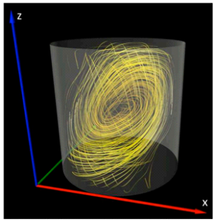
Figure 1. Global flow conditions in inhomogeneous convective experimental turbulence.
It is important to note that their results hold for three turbulent flows of increasing complexity and they “get a sense of the mean wind, or large-scale circulation, that exists in the flows consisting of a single circulation roll that fills the whole cell (Figure 1) and obeys very slow dynamics with respect to time, which would require very long simulation runs, inaccessible with present capabilities” . One can expect these results to be universal, but the utility of them in large-scale forcing in homogeneous isotropic turbulence (studying intermittent or anomalous scaling properties of turbulence) is not properly understood. Experimental results obtained in the great experimental aerodynamic tunnel of Modane (France) show that “the probability density functions (PDFs) of velocity increments undergo a continuous shape deformation, starting from the integral length scale L at which statistics can be considered as Gaussian, down to the dissipative scales where the PDF is highly non Gaussian“ . This phenomenon is a manifestation of the intermittent nature of turbulence as indicated by Kolmogorov and Obukhov . In this investigation the velocity increments, focused on two-points quantities, were fully determined by the corresponding probability but “Nothing is said on the long range correlated nature of velocity…It remains to propose stochastic processes able to reproduce velocity statistics in the intermediate and dissipative ranges” .
That is, the reality is more complicated than what we get from a highly averaged description of the turbulent flow. To illustrate the point, the measurements of stresses in a classic Taylor-Couette experiment flow show that the laminar regime is given by the horizontal line, with the Reynolds number increasing from right to left, and the turbulent regime is given by the (almost) vertical line. In spite of the beauty of this result, “detailed inspection of the flow for different rotating velocities of the inner and outer cylinders shows a complex situation” , the experiment showing also an example of the spatial intermittency in which turbulence appears in spots surrounded by quasilaminar flow. This flow, like any flow in a finite container, may be “extremely conditioned by the details of the external stresses imposed on the flow as well as by the geometry of the container” . Possibly, this is not real turbulence like the fully developed turbulence is, which is free to develop without imposed constraints while the small scales almost always obey Kolmogorov's universality.
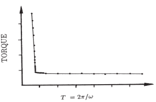
Figure 2. Experimental measurements of the torque exerted by the fluid on the lateral walls of a Taylor-Couette apparatus as a function of the rotation period. The inner cylinder rotates and the outer one is at rest. The period provides a measure of the Reynolds number of the flow.
The displaying of the interactions that characterize the turbulent fluctuations constitutes the famous energy cascade process described by Kolmogorov. The energy spectrum as a function of the wave number follows a power law (-5/3) over a range of length scales (i.e. the inverse of wave numbers) extending from the integral scale to the dissipation scale. Turbulent flows may show the same energy spectrum indicated by the power law and be produced by different mechanisms acting at different scales. For example, Frisch , pag. 80] noticed that “In the atmosphere of the Earth there are a number of instability mechanisms acting on very different scales: for example, the large-scale baroclinic instability and small-scale convective instability. Under what conditions can the resulting turbulent flows coexist?” This question is important in view of a possibility of increasing the weather predictability, as Lorenz argued , based on the Kolmogorov theory. Indeed, “ the local power law appeared in fact to hold instantaneously (not only deterministically for individual flow realizations), without smearing in time, beyond what could be proved mathematically and with the stringent condition that the local Reynolds number must be high”, as reminded by Eyink . The phenomenon of turbulence has been studied in detail using the principles and concepts put forward by Kolmogorov, but “is also evident that we are still too far from grasping a number of randomized and chaotic behaviors that are exhibited by fluids….a number of facets and aspects of his propositions do not fit well with the actual turbulence” and thus, to examine and develop as many as necessary experimental studies. Frisch and Parisi show that a simple way of explaining power law structure function is “to invoke singularities of the Euler equations considered as a limit of the Navier-Stokes equations as the viscosity tends to zero”. They show that in the fully developed turbulence regime, “the function d(h) of the Hausdorff dimension for the set of points for which the velocity field has a singularity of order h … is nontrivial and singularities of different kinds, if they exist, are concentrated on sets having different Hausdorff dimensions”. I think this is important if we see that d(h) has a “clear dynamical meaning because it contains most of the relevant information on the scaling laws for fully developed turbulence”. It would be rather important to measure accurately d(h) and to find good evidence for its universality (independence from the initial conditions).
In one of his papers in 1949, Kolmogorov stated that the accelerations of particles in turbulent flow must be determined principally by small-scale perturbations (in contrast to the velocities, in which small-scale perturbations bring about only a very small contribution) and that “for a significant average velocity of flow U, these accelerations will be very large (since, with growth of U, the mean square acceleration w grows proportionally to U⁹⁄⁴ (footnote 1, pag. 102). The approximate calculation, performed afterwards on the suggestion of Kolmogorov, completely verified this assumption: ”it was found, for example, that in the ground layer of the atmosphere for rather strong wind, w may exceed completely the acceleration due to the force of gravity g” ibidem]. Large fluctuations of the acceleration are evidenced by calculations based on Eularian dynamics and also seen in records of velocity fluctuations in a high speed wind tunnel. Pomeau and Le Berre observe that the fluctuations “do not happen all the time, but are strongly correlated to sparse large velocity fluctuations” and conclude that “such a correlation contradicts Kolmogorov scaling law” . The idea of reconsidering the scaling laws for turbulence from this observation is iconoclastic and for the time being excessive. More experimental data are needed. For example, La Porta and al. show that: “ the acceleration of a fluid particle in a turbulent flow (turbulence was generated between coaxial counter-rotating disks in a closed flow chamber) is an extremely intermittent variable - particles are observed with accelerations of up to 1,500 times the acceleration of gravity (equivalent to 40 times the root mean square acceleration). We find that the acceleration data reflect the anisotropy of the large-scale flow at all Reynolds numbers studied”. It is necessary to refer here to the scaling framework for complex atmospheric turbulence. Using Monin-Obukhov similarity theory (MOST), Stiperski and Calaf improve the approach based on anisotropy. Their results show that “while anisotropy itself is site, stratification, and scale dependent, its role in the generalized scaling is that of a unifying variable”.
We have to believe that an improved understanding of turbulence contributes to a new ability to predict phenomena in the area of environmental physics. For example, we may suppose that some rare atmospheric environment or the possible relationship between the global anisotropy of the physical space and the occurrence of the most violent tornadoes, is capable of creating the conditions for those natural huge energy levels. The destructive energy of tornadoes is comparable with the energy of nuclear explosions while numerical simulations of real tornadoes suffer from significant underestimation of their intensity. Baurov and al. also observe that:”Despite the intrinsic huge complexity and chaotic nature of the atmosphere at any scale, on the basis of (our) analysis… it is possible to state that the most powerful tornadoes can occur only at specific times of the day which depend on latitude, longitude and day of the year”. The fact is that the dissipation of energy itself in a turbulent flow will also be a random variable and because of the disorder of the process of the transfer of energy from the largest disturbances to the smallest we should expect that for unbounded growth of the Reynolds number the dispersion of that energy dissipation rate will grow unboundedly (pag. 103). Generally speaking, every approach to the theory of turbulence, starting from the consideration of the probability distribution of the ratios of the differences of velocities, needs considerable further development. The complete unfolding of these approaches requires much more than the similarity hypotheses may be able to give. In fact, if, in the study of hydrodynamical fields of turbulent flow, we are concerned only with the existence of some universal probability distributions of random fields, “naturally arises the problem of finding explicitly the corresponding universal distributions, which is incomparably more difficult than the problem of establishing conditions for which also the universal distributions exist. Thus, the theory of similarity does not remove from the agenda the general problem of turbulence” (pag. 105).
Identity transitions are a natural phenomenon which we should understand better in order to better understand reality. Modelling of admixtures transport is carried out on the basis of systems of diffusion equations with coefficients dependent on parameters of atmospheric turbulence. It should be noted that modelling of air flows in the boundary layer of the atmosphere is a complicated problem, the solution of which depends on the theoretical ideas about turbulence. The relatively high frequency of occurrence of turbulence near the ground is one of the characteristics that makes the boundary layer different from the rest of the atmosphere. Outside of the boundary layer, turbulence is primarily found in convective clouds, and near the jet stream where strong wind shears can create clear air turbulence. Global warming influences the position of the jet streams although the exact mechanisms are not yet known. Observed real jets show that: “under natural conditions the jet stream has a very important role in creating really extreme weather conditions” .
The questions of the physics of the surface layer have a general geophysical significance, since the dynamic interaction of the atmosphere and the substrate, the “feeding” of the atmosphere by moisture and heat, is realized through the surface layer. A simplified parameterization of planetary boundary layer through Monin-Obukhov similarity theory (MOST) in all weather, climate, ocean, and air pollution models “has become one of the most celebrated theories in the atmospheric boundary layer” . Conclusions derived from the MOST are the principal tool for calculating the characteristics of the turbulent atmospheric surface layer. Also, in calculating the turbulence of the main space of the atmospheric surface layer at a distance above sea level greater than a few times the height of the largest waves. The mean vertical profiles of wind speed, air temperature, and humidity are described by this theoretical (logarithmic) form which, in addition, depends on the roughness parameter of the underlying surface or the roughness length scale of underlying surface. Yet, the disturbances, induced by waves, cause strong influence on the dynamics of this layer. As pointed by Benilov: “The effect of this factor shows up in all characteristics of turbulence and is still poorly understood” . This approach cannot be realized in solving the problem of transport of admixture in the lower layers of the atmosphere. Monin and Obukhov indicate that its applicability is limited, among other things, by “the general breakdown of scaling for intermittent turbulence, where the presence of so-called submeso motions requires alternative approaches” . The transition from the laminar flow to the turbulent flow is a very attractive phenomenon from the mathematical point of view. The initial laminar flow, which is not consisting of any chaotic waves, suddenly transforms in a state with a chaotic behavior. This problem of transformation called "dynamical chaos" has been investigated by many authors. “The theory of the "dynamical chaos" is based mostly on the analyses of the simplifier dynamical systems (Lorenz-like chaos) which can't be used directly for the boundary layer problem. The turbulent boundary layer is characterized by chaotic pulsation of the flow parameters. The surface which separates the turbulent stream from the outer flow looks like a rough surface” .
A close analogy between the theory of turbulence and the quantum theory of fields appears once more here, allowing the hope that significant steps in one of these branches may prove a real help in the development of the second (pag. 106). For example, the strength and size of the vortex are crucial for generating interactions in real flows between the vortex and the rest of the close fluid environment that are significant enough to observe both in quantum fluids and tornadoes. And, as the relationship between mathematical theory and reality is nowhere near straightforward for quantum objects, something similar (less strong probably) is observed in "weird" turbulent phenomena. Or, the similarity between a larger and larger number of atoms displaying the quantum effect and an increased number of vortices displaying the pulsation pattern. Quantum objects, at the smallest of disturbances, lose their fundamental properties, i.e. ”entanglement vanishes and superpositions collapse - and the larger an object is, the more likely it is to succumb to certainty” . Turbulent fluids are in a sense as unpredictable as the quantum objects, the ” boundaries” of which are melted into one another and may be in this way producing intermittency (an alternance of calm periods and bursts of intense activity for accelerations or velocity increments) and coherent structures (eddies preserving a certain spatial organization downstream the separation of a boundary layer). Intermittency and coherent structures were presented earlier in this paper and one can easily compare and acknowledge the similarity of definitions. They show something like a fundamental scaling up and a threshold, both in quantum and turbulent phenomena. We are aiming to understand the physical mechanism of processes occurring in nature, even if this requires going outside the limits of the original logical schemes.
Turbulence is a multi-scale problem with a highly non-linear coupling between the scales. The non-linearity here, as in any dynamic system, is responsible for the difficulties arising in the attempt to obtain an accurate prediction of turbulent flows. They are out of equilibrium systems. Turbulent flows are neither deterministic nor fully random: “high-Reynolds number turbulent flows are far from being totally disorganized…. large-scale eddies in a flow past an obstacle (a sphere, for example) preserving a certain spatial organization are called coherent structures and retain their identity for much longer times than the eddy turn-over time characteristic of the turbulent fluctuation.” . Frisch suggests that coherent structures may play an important role in the dynamics of atmospheric turbulence and concludes: “If this is so, predictability estimates based on turbulence phenomenology (à la Kolmogorov) may be very misleading”. Defining the kinematical properties of hydrodynamical fields through the mathematics of random functions is not enough. From a physical point of view, the equations of dynamics impose deeper important limitations. There is no simple linear relation between the turbulent behavior and its representation. Turbulent flows at large Reynolds numbers display such complex behavior in space and time that it is impossible to obtain a solution of the fluid equations properly representing the flow field in such situations. This makes necessary a statistical description of the fluctuations in those flows. The previously mentioned explanation (in the Introduction subsection) about the practical utility of the Kolmogorov’s assumption of turbulence space distribution is questioned by Pomeau and Le Berre : “Kolmogorov suggested using the dissipated power per unit mass on average as a scaling parameter for the statistics of turbulence, assumed to be homogeneous and isotropic. Even though this last assumption is done very often in theoretical works, its relevance to explain physical situations is far from obvious. Specifically, most turbulent flows, if not all of them, have a geometrical structure making them non homogeneous and non isotropic”. Turbulence produces gradients and vorticity and the rate at which energy is dissipated is particularly pronounced in regions where the instantaneous velocity gradients are large, e.g. in the smallest eddies. For instance, of practical importance is the fact that vorticity flux from the body surface can be directly related to drag.
One of the main unsolved properties of fully developed turbulence is intermittency. More specifically there is still no explanation grounded on properties of the fluid equations for the observed intermittency in flows at very large Reynolds number. Investigating the role of intermittencies in real fluid turbulence, Pomeau and Le Berre have shown that the fluctuations of the solutions of the “inviscid” Euler equation for an incompressible fluid display strong analogies with real fluid turbulence: “In particular, they exhibit a well-defined Kolmogorov spectrum in an “inertial range” between the injection at large scales and dissipation at small scales.” This shows that “the occurrence of singularities for the “inviscid” part of the equation of motion is a way to explain both how dissipation and intermittency occur in such a turbulent system.” If in the atmosphere there is an energy spectral gap (and turbulent flows coexist being separated by this gap), “It could be that the gap in the energy spectrum is filled by rare but violent meteorological events and does not exist in the mean” . Experimental and numerical investigations of wall-bounded turbulence at high Reynolds numbers have observed the so-called “extreme events” when the necessary condition of the uniform vanishing of wall-normal velocity is breaked down, also associated with skin friction showing an abrupt boundary-layer separation. They are even more extreme in other flows such as movement past a sphere or in a hydraulically rough pipe (pag. 57).
I use as a partial conclusion Eyink comment about the “building block” flows, under the subtitle How Do We Check If It’s True?: “It is far from clear that any of the previous “simple” flows (“canonical wall-bounded flows”- plane-parallel channel flow, smooth pipe flow, and flat-plate boundary layer) are a good starting point for understanding more realistic wall-bounded turbulence in general” (pag. 59). As a rule we observe that turbulent flows are dynamically complicated in natural environments, displaying a variety of spatial and temporal features. The real problem is then if we can treat them mathematically as fully developed turbulent flows using the Euler equations considered as limits of the Navier-Stokes equations as the viscosity tends to zero. We know that the occurrence of extreme meteorological events is strongly related to the intermittency in spatial turbulence structures, with an evident dependence on the spatial scale. Direct numerical simulations also revealed a non-linear feedback mechanism.
Recently, Yu Deng et al. took, somehow unexpectedly, Hilbert's conjecture approach to axiomatically derive the laws of fluid flows, i.e. the incompressible Navier-Stokes-Fourier system from Newton’s laws. Hilbert suggested in 1900 "to treat in the same manner, by means of axioms, those physical sciences in which already today mathematics plays an important part; in the first rank are the theory of probabilities and mechanics" and, using Boltzmann’s work to pass “from the atomistic view to the laws of motion of continua" [quoted in . The main and interesting idea of the authors is to connect the kinetic limit to the hydrodynamic limit and to obtain a full derivation of the fluid equations. The math is performed on a microscopic system formed of N particles of diameter ε undergoing elastic collisions. The kinetic limit is the one in which N → ∞, ε → 0. The hydrodynamic limit is the one that derives the equations of fluid mechanics (like compressible Euler, incompressible Euler, incompressible Navier-Stokes etc.) as appropriate limits of Boltzmann’s kinetic equation when the collision rate α is taken to infinity. The fluid velocity and density are obtained by “directly taking limits of the associated statistical quantities coming from the hard sphere dynamics”. In the derivation of fluid equations the authors indicate, for example, that “ the velocity truncation … is merely for technical reasons, and is also natural from the physical point of view” . A fundamental difficulty in this approach “is the passage from the time-reversible microscopic Newton’s theory to the time-irreversible mesoscopic Boltzmann theory”. In a substantial and apparently consistent mathematical development, the authors show several results, including the passage from colliding particle systems to the compressible Euler equation. For now it is hard to see how this approach may be of practical use in turbulent flows. But, as we tried to explain in this article, there is very much needed new imagination in the calculations of turbulence. In science there is an assurance out-of-nowhere, that is, solid results that appear unexpectedly but due to a large amount of accumulated knowledge.
3. Extreme Weather Events Modelling and Natural Observations
A real-physics climate dilemma is whether to use predominantly climate extreme events models based on physics or solving climatic models using AI (machine-learning) based on data. We should have both ways: new physics/models and extrapolate historical data. Chaos and order co-exist in the weather and climate dynamics. Based on observations of local spectra characteristics, Serykh and Sonechkin conclude that “the dynamics consists of a mix of partly chaotic and partly ordered weather variations”. The weather could be chaotic while the climate is not. Weather and climate prediction should use different models. When the existing models do not engage in solving complex and also excessively complicated physical problems, the existing historical data and observations can be evaluated. Equations calculate with the certainty that is fundamentally included in theoretical knowledge, while statistics deal with probabilities, i.e. uncertainty. That is essentially the cause of the weak overlapping between theoretical models and statistical treatment of the recorded data. Another problem involved in this disparity is that describing extreme events using sophisticated mathematical quantities should take into account that sometimes these “do not commute”, in the sense indicated by Carlo Rovelli , i.e. the multiplication of two quantities gives a different result depending on which comes first. I think of the utility, if not the necessity, of transposing, at least conceptually, the concepts of mutual information and consensus in quantum models into the study of turbulence. Mutual information would then be the one that captures the overlap between what we learn from theoretical models on one hand, and from climate extreme events studies on the other, until a consensus is reached. This is not common practice for now although overlapping of events and interfering properties and imprecise meanings are abundant. It would be a kind of framework for understanding, merging information and forms, because, evidently, it is not just a correlation. For instance, when the different natural features are present and filling a certain sufficiently large space in the atmosphere, subtle correlations may be overwhelmed. The problem is if we have gathered enough information to arrive at the same conclusion about the turbulent state of the system (natural or experimental). We examine the agreement and the context of the data (observations). We expose the flaws of the theoretical models while showing how important are the achievements. Clearly we think it should incorporate more of the physics, as Gavin Schmidt noted: “Weather and climate are based on physics” . AI makes evaluations and runs simulations but are “inflexible and often vague”. Underlying physical processes are not yet understood and also, representing them is very costly (computational resources). Interactions at play between the atmosphere, oceans, and land such as how heat flows through ocean eddies. Numerous interactions between the components of the climate system and non-linear feedback loops induce random fluctuations on various time scales. The recent catastrophic event in Valence (Spain), called “gota fria”(cold drop), is one of the most clear proofs of erratic weather dynamics depending on multiple factors, as the ambient temperature (which is energy), humidity, pressure, winds, orography and other geographical and atmospheric elements. The winds from the East and the abnormally high temperature in the surface waters of the Mediterranean Sea repeatedly generated the accumulation of water in the storm. The mountains in the vicinity of the coast pushed up the humid and warm air, establishing a constant cycle. How to formulate a viable theoretical prediction model under such a very complicated conjuncture? None of the above-mentioned factors are predictable in larger than 24 hours. The limits of prediction are two-fold. On one hand the amount of humidity and the temperature gradient and the resulting winds, on the other. Warmer air captures more humidity (like a hair-dryer). Paradoxically, this is aggravating both droughts and floods. Indeed, recent studies show that: “when it is not raining, the warm, dry air is absorbing humidity, increasing the drought intensity. When it is raining, the atmosphere is more humid, increasing the intensity and duration of rains” . With a large amount of data of these parameters combined with a powerful scientific intuition there is a chance to overcome, at least partially, the pure unpredictability of an event like the one in Valence.
Often we speak about a significant level of uncertainty. What is significant? What we have is the signature of climate and weather. If a climate pattern seems to be firmly established we have still to guess if the physics (unknown in its totality) could undermine that solidity of the pattern. For example, what the local conditions might be and how they might change over time.
Statistical uncertainty is a measure of uncertainty of the time average with respect to the unsteadiness of the flow or surface pressure field. Therefore, it is highly important to verify that the time average of a statistically, stationary stochastic process (such as a tornado) converges against the mean value of all possible realisations within the chosen measurement duration. For instance, full-scale measurements in tornadoes is extremely difficult considering the instabilities, singularities and non-linear effects present in real events. Indeed, “Measured flow patterns are far less structured and organised than the pattern suggested by any of the vortex models. Some vortex models are able to represent certain flow patterns at certain heights but fail, due to their simplifications, in replicating the entire three-dimensional flow structure obtained experimentally” . It is certainly important to study the essentially unknown initial stage of whirlwind and tornado origination. This stage is considered to be an “explosive instability” in nature. Already in 1915, G.I.Taylor, describing the eddy motion in the atmosphere, thought that “...a very large amount of momentum is communicated by means of eddies to the ground”. A possible connection between tornadoes and vorticity proposed in is that “vortices stir or pump the tornado and increase the vorticity…the frequency, strengths and stretching of the vortices determine the eventual strength of the tornado”. The growth of vorticity in whirlwinds and tornadoes may (under certain conditions) proceed exponentially, which is typical for explosive instability, as suggested in . The vortex intensification leads to a critical threshold which we may suppose is the mechanism transforming a tornado in a large single vortex undergoing a breakdown as indicated in . Turbulent flows at high Reynolds numbers are investigated by laboratory experiments and by repeated numerical simulations in order to understand what we cannot properly measure, like for instance the features of the vortex motion. From a mathematical perspective, the turbulent movement is described by vorticity. The notion of an “eddy” or “whorl” is naturally associated with the idea of a vortex, well imagined in a tornado, for instance, but this association does not prove to be useful in combining mathematical approach with physical reality. In particular, the vortex breakdown and the onset of spatial instability in the dominant flow dynamics. If a tornado is a “highly convergent swirling wind affecting a relatively narrow path” and “the turbulent energy is mainly generated by radial straining. The location of the maximum turbulent production is close to the ground inside the core region of the tornado vortex. Most importantly, the maximum turbulent kinetic energy is produced at a swirl ratio which corresponds to the tornado vortex touch- down. This leads to the possibility that turbulent energy rather than mean velocity relates to the intense destruction that tornadoes produce at the ground level” , it is important to introduce the experimental results from the study of swirling jets. In particular, the vortex breakdown is occurring when the swirl intensity exceeds a certain threshold . In the case of tornadoes, the main scale corresponds to the average wind speed in the tornado (a core formed by a primary jet) while the intensification of the vortex is accompanied by an acceleration of air rotation in the center. In the study of the essentially unknown initial stage of a tornado, for instance, Arsenyev and Eppelbaum state that:“The most prevalent methods for modeling catastrophic atmospheric events….can be reduced to two approaches: (1) statistical based on the probability density function and (2) deterministic based on the complex numerical solution of systems of differential equations for atmospheric and ocean dynamics” . Nechayev and Solovyev tried to explain unusual hydrodynamic phenomena (paradoxes) in the framework of classical hydrodynamics, using its basic laws in a simplified model based on the air density decrease in ascending jets. Another, stochastic, small scale model , explains the small-scale turbulence which needs to be correlated to the idea that the jet in the central core effectively connects atmospheric layers with different air densities. Yet, as shown in , “In the presence of atmospheric cyclones carrying strong winds, clouds and precipitation, eddies of medium mesoscale (intermediate between the main macroflow and small-scale turbulence) appear in the turbulent flow. Instability and growth of the mean flow arise due to the fulfillment of the unique conditions established by the mesoscale turbulence theory.” And another way consists in calculating the vertical and tangential profiles through the tornado vortex simulation in numerical studies. The model used in considers “axi-symmetric flow in a cylindrical region of moist, conditionally unstable air, initially in uniform rotation at each height and increasing in strength with height” and “rotation (that) is imposed by prescribing a swirling velocity component on air entering through the radial boundary, whereas the initial rotation in the flow domain is everywhere zero”. It does not use hydrodynamic equations and does not sufficiently relate the results to tornado observations. Tsinober insists that the “vitally important part of the physics of turbulence resides in the unresolved small-scales” and that we cannot disregard the possibility that the all important properties of the resolved large scale “do not depend essentially on what happens in the unresolved small scales”. The important fact is that the dissipation of the turbulent energy takes place within the vorticity turbulent movement, closely related to “the form of the turbulent region (which) is shaped by the properties of the movement in the (core) fundamental volume of the fluid” . This observation could play a decisive role in natural fluid movements. A theoretically complete and practically useful model for determining this shape, based on the Euler equations, doesn’t exist now. Indeed, the interacting eddies in turbulent air and liquid flows become chaotically complex in short laps of time (fluctuating very high acceleration of fluid particles occurs in milliseconds) . Thus, precise simulation is impossible for even the most powerful computers, either by solving hydrodynamic equations or probabilities . The solving of the weak Euler solutions (which are mathematically equivalent to the “coarse-grained solutions” that are used but do not change any physical reality), imply a filter decomposition, i.e. an arbitrary choice of a technical nature. Evidently, as remarks Tsinober:“After all Nature may and likely does not know about our decomposition” . Serious improvement in both the algorithm and its implementation (in both large-scale deterministic and probabilistic simulations), using a variety of direct computational approaches, is needed. Ideas moving back and forth between theory and natural science, learning from experimental observations and understanding of the physics of how turbulence works.
Much of the boundary layer turbulence is generated by forcings from the ground. For example, solar heating of the ground during sunny days causes thermals of warmer air to rise. These thermals are in fact large eddies. Frictional drag on the air flowing over the ground causes irregular shears to develop, which frequently become turbulent. The largest boundary layer eddies have sizes roughly equal to the depth of the boundary layer; that is, 100 to 3000 m in diameter. These are the most intense eddies because they are produced directly by the forcings. Observations show frequent lack of turbulence above the boundary layer which indicates that the rest of the free atmosphere doesn’t respond to surface changes. In fact, the free atmosphere behaves as if there were no boundary that plays a role in it. It doesn’t mean that wind flowing over the top height geometry is not an agent of the turbulent dynamics. The turbulent boundary layer is characterized by chaotic pulsation of the flow parameters. The surface which separates the turbulent stream from the outer flow looks like a rough surface. The questions of the physics of the surface layer have a general geophysical significance, since the dynamic interaction of the atmosphere and the substrate, the “feeding” of the atmosphere by moisture and heat, is realized through the surface layer. For example, the violent, atypical, discontinuous nature of rare events (an alternance of probability peaks and of almost empty minima in the velocity PDF of individual segments) are associated with the intermittent behavior of turbulence indicated by probability distribution functions (PDF) of the turbulent velocity signal and by “the existence of very large tails of the acceleration probability distribution function, which have been experimentally measured up to more than 50 standard deviations” . The mutual adaptation of air pressure and wind velocity to each other results in the tornado appearance in which the wind velocity and the air pressure gradient can reach huge values. For example, in the violent tornado in Oklahoma City (USA) on May 3, 1999 (48 people died), according to Monastersky (quoted in ), the maximum wind velocity was 512 km/h. The maximal drop of the air pressure in the tornado is not large, about 50 hectoPascal. However, according to the equation of the rotating vertical air column based on the cyclostrophic balance, “the wind velocity inside a tornado is determined by the radial gradients of the pressure (but not by the pressure itself). Thus, sharp spatial variations of the air pressure inside a tornado can induce a strong wind” . This work takes into consideration another essential parameter which is the vorticity. The calculations and the measurements demonstrate that the radial distribution of vorticity in a F5 tornado is maximal in the tornado center, attaining a very high value of 15 Hz, while at 27 km from the center is less than one Hz.
The development of turbulence physical models are necessary in order to be effective enough for tornado generation forecasts. Thus, “The macroscale air circulation can be described as the suction of the surface air from the periphery towards the tornado center. Then, inside the eyewall, the air masses ascend till about 1 km height where they diverge to the periphery and descend. In this way, the tornado structure is created . The main feature of the mesoscale turbulence theory is that three scales of motion of the environment are considered. Global macro scale L (middle flow), meso scale m and micro scale l (small-scale turbulence, in which energy is dissipated into heat). Meso scale corresponds to the presence in the flow of rotating vortices having their own spin (angular velocity of rotation) and moment of inertia. Meso eddies interact with small-scale turbulence and with the average flow. Under some specific conditions they can transmit energy to the middle flow, strengthening it. Then, inside the eyewall, the air masses ascend till about 1 km height where they diverge to the periphery and descend .
There is little indication that tornados will become less unpredictable in the near future. By analogy, let’s remember that although we have a fairly good idea about the physical mechanism that triggers an earthquake, we are not able to predict neither the occurrence nor the amplitude of such an event. As in any random natural event, improvements in better understanding the tornado dynamics related to tornado formation (obvious necessity for prediction and warnings) are needed. Such efforts are complicated by the fact that tornadoes are of short duration, and they occur relatively infrequently, irregularly, and in different geographical locations each year. In the scientific production on extreme weather events we note that there are relatively few common references in scientific papers in the different approaches of the hydrodynamic calculations of turbulent vorticity. From this point of view, the remark made in 1982 , that “many aspects of tornado dynamics remain uncertain or unexplained”, is still largely valid.
Reconnecting with the theoretical foundations, it is useful to remember that Kolmogorov made important contributions to the Taylor turbulence theory (mentioned earlier in this article). He suggested : (1) To avoid the isotropy of the velocity pulsations fields but to save it for the pulsation differences. His local isotropy was a great step towards the other cases of mean velocity fields besides the constant velocity (in 1941); (2) To consider the energy flux as the main parameter of energy cascades in turbulence (in 1941), coinciding with the Schrödinger principle for thermodynamically open systems and (3) To introduce the rotation frequency as an additional kinematical parameter (in 1942). These obviously important suggestions remain largely outside the current calculations of extreme weather events.
As concerns the intermittent bursts, for instance, they are predicted to result from “quantum jumps” between the probability peaks, when the particle velocity crosses the zero minima, involving a divergence of the acceleration component. The quantum behavior traits of contextuality and nonlocality could play in a similar way in turbulent flows. The realm of the so-called Statistical Turbulence Theory where “in the statistical averages much of the information that may be relevant to the understanding of the turbulent mechanisms may be lost, especially phase relationships” does not offer a sufficient understanding of turbulence as a natural phenomenon and so, in order “to understand highly intermittent turbulence production mechanisms for which intricate phase relationships are likely to play an essential role, standard averaging techniques are insufficient”.
Nature is essentially non-local. In the meantime we don’t know where the boundary lies between quantum and classical physics. Probably the universe doesn’t tend towards disorder, as indicated by the entropy law, but towards complexity. We need to find a deeper theory.
The picture of turbulence in natural events described in this article (far from being a resolved puzzle) would not be reasonably completed without two other features: electric force and clouds.
Various works point to a possible association between tornadoes and luminous electrical phenomena . It seems that the whole range of energy inputs may have (or not) an important impact in the process of triggering tornadoes. Currently we are unable to predict the time-length (minutes to hours) or the intensity of the tornadoes which point to the presence of one or more physical robust thresholds in the system. Once the threshold is exceeded we have a tornado. On the contrary, in the case in which there is no such threshold a tornado doesn’t occur. Maybe under some conditions - which we don’t know comprehensively today - atmospheric turbulence is pushed into a kind of collective state, let’s say a “resonating structure” creating a bond of vorticity. For example, Rasmussen and Blanchard found that “a certain amount of boundary layer shear in conjunction with a certain level of convective available potential energy is required for a tornado to occur”. These assumptions also suggest that since there are various trigger mechanisms for tornadogenesis our predictive ability is even less consistent with the assembly of existing data. We are currently unable to provide a solid grounded correlation between global warming, climate change, and tornadic activity. The existing data for tornados on a large scale start in the 1970s and it is necessary to have and thoroughly examine more decades of data.
Another very important factor in the dynamics of climate change is the presence of clouds in the atmosphere along with winds and precipitation. We are far from being capable of determining the balance between how the clouds reflect the sunlight and in the mean time trap the warm or cold air below :“This balance makes clouds the biggest unknown in predicting future climate change”. This statement refers to the slowly varying and constant evolution of climate changes mentioned in the introduction of this article. Studying the real clouds' feedback in greater detail is the way to understand the formation of stormclouds which are sometimes responsible for extreme events. Such studies necessarily have to measure the shape and type of aerosols because, as indicated by Graham Feingold: “the other major source of uncertainty alongside these cloud feedbacks is the role of particles suspended in the atmosphere” . Climate scientist Kara Lamb says that: “we can model maybe a single cloud or a field of clouds with relatively high accuracy, but if you want to take that and put it into a climate model, you have to simplify it a lot more . Nevertheless, the numerical cloud-resolving models with high resolution are a promising tool although they require so much computing power that they can only make near-term predictions or simulate limited areas. In my opinion it is evenly important to correlate in-situ studies of clouds with in-situ measures of turbulence parameters. Indeed, in the presence of atmospheric cyclones carrying strong winds, clouds and precipitation, eddies of medium mesoscale (intermediate between the main macroflow and small-scale turbulence) appear in the turbulent flow. Their role is delineated in this work in the previous paragraph.
4. Conclusions
The motivation of this article is that we should achieve a better understanding of why the respective fields of climate (extreme events) models and theoretical mathematical models of turbulence physics are not sufficiently if not even essentially overlapping as they could be normally. In both fields of research which are dedicated essentially to the turbulent features and the non-linear dynamics of fluid flows we are confronted with the problem of chaotic behavior and resolving mathematically the observed realities of collapse and intermittency of the coherent structures of turbulent flows. Although the profound nature of turbulent behavior is not yet comprehensively understood, there is no valid reason for the apparently rather distinct approaches in those two research fields playing on the same fundamental object of study. Let’s call this situation a “binomial puzzle”. The transportation processes in turbulent flows, which are in fact ingredients of the dynamics of the extreme events, constitute a real and strong link between the investigation of turbulence and that of the extreme events. The problem raised in this article is quite simple but might have at this stage a complexity to the solution. If the mathematical techniques are not yet the appropriate ones or haven’t been developed, progress in the area is not possible with calculus. This is a reason for the above-mentioned overlapping. In what sense mathematical exact results approximating real flows are representing useful solutions for real natural extreme events? Today we understand better that studying turbulence and focusing on advancing in the theoretical field essentially using Kolmogorov’s thinking, should be substantially more complemented by the applications in different fields. Increasing or refining the investigative instruments that mediate between theory and the world. Epistemic objects (defined as focal points of knowledge) are unstable entities existing at the boundary between the known and the unknown, or between epistemic and technical objects . Technical objects (created for various purposes like design, engineering or science) provide a stable context for experimentation. They can be material objects, concepts, systems of accepted knowledge, or instruments. They work as necessary tools capable of producing valuable and verifiable answers about epistemic objects: “When modelling is used for gaining knowledge about a (partly) unknown object the process is not an approximation to something already stable. New research objects are unstable in the sense that their properties and boundaries are neither known in advance nor directly accessible for observation.” . I think that this epistemological approach is appropriate in my inquiry on the weak overlapping of turbulence theoretical models and extreme events studies. Models, as shown in this paper, involve complex relations and need to primarily focus on non-linearities of the relation between the object under study and its representation. Enhancing stability of the models when dealing with unstable features is important for understanding the role of models in research since models are the essentialization of the real phenomena in order to generate knowledge about what is not yet known. They forcibly display an unstable part that eventually may produce not just the expected results but also unpredictable results. In that sense, “modeling is not a matter of accurately representing targets but of generating, manipulating and superposing different epistemic tools to learn about what is not yet known..
A powerful tool of extending simulations of the climate events is becoming more and more useful as supercomputers can generate virtual observations. Indeed, instead of putting the emphasis on traditional statistics based on measuring the uncertainty of inferences under restrictive assumptions, scientists from the Met Office in Britain, were able to simulate thousands of possible weather scenarios and understand what actually happened in weather evolution, including extreme events. As a matter of fact, we can form reasonable beliefs according to a rule of inquiry that is certain to be correct under a set of assumptions, but we may be wrong if the assumptions are false. There is no guarantee we converge to the truth eventually and even less as to when. As Thierry Corti, a climate-risk analyst, observes, “the risk landscape is evolving. So if you simulate probabilities of a rare event you need to take that against the backdrop of something that’s changing. That makes it much more complex.” In the scientific investigative sense, a repetitive computational cycle was generated adding a “chaotic-like” input in the form of a small and local amount of heat. The recorded (present) climate was perturbated each time in intervals of minutes and thus a range of virtual winters including extremes was generated. In the case of floods, the research group found a 34% chance each winter that rainfall records would be broken in at least one of four broad regions of Britain. In the end, there were one hundred times more possible simulations of the current climate than is available from real observations. “Whilst statistical methods exist using observations alone to estimate the risk of record rainfall, our new technique allows us to give a more precise estimate for a one-in-100, or one-in-20 scenario.” .
Climate adaptation will involve preparing for the deeper droughts, extended heat waves, extreme precipitation, extreme storms, bigger wildfires, and sea-level rise that accompany rising temperatures. It is clearly required to improve climate modeling and better predictions. The uncertainty of where and when climate events will occur adds to the adaptation challenge. Existing global climate models are at too large a scale to provide localized guidance, providing only general information about trends across broad landscapes. The prediction of local events needs to be better served by an interplay between theory of physical processes and experimental research, overlapping the modelling of fundamental understanding of turbulence and of real extreme events.
This work isn’t intended to compose a kind of anthology of turbulence. There are several valuable works in that sense . We try to understand if some unity can be found.
We want to know what theory helps the advancement of knowledge in turbulence and in the meantime we want to know what’s the technique to use; both theory and technique based on reality.
We need redundancy for error corrections. Overlapping offers direction for the research. The path of research which includes unknown orientation, errors, incomplete coverage, constraints and repeats of the calculations show the analytic as well as experimental difficulties. It is broadly observational science vs. structural chaotic features of turbulence.
Horace, more than two thousands years ago, observed: Naturam expellas furca, tamen usque recurret (You can get nature out of the way with a fork but she will always come back) and Newton: “The concept of miracle does include unusualness. Think of things we count as ‘natural’ although they are absolutely wonderful and manifest enormous amounts of power. Astounding as these are, they aren’t miracles, simply because they are common, usual. But it doesn’t follow that everything unusual is a miracle. It might instead be only an irregular and rarer effect of usual causes” .
Conflicts of Interest
The authors declare no conflict of interests.
References
[1] Uriel Frisch, “Fully developed turbulence and intermittency" in “Turbulence and predictability in geophysical fluid dynamics and climate dynamics”, Proceedings of the International School of Physics Enrico Fermi, North-Holland, 1985, pag. 84.
[2] Josep M. Massaguer, “From pre-turbulent flows to fully developed turbulence” SCI. MAR., 61 (Supl. 1): 63-73, 1997.
[3] J. O. Hinze, “Turbulence”, MCGraw-Hill Book Company, 1959.
[4] Townsend, A. A., “The Structure of Turbulent Shear Flow”, Cambridge University Press, New York, 1956.
[5] P. Manneville, “Systèmes dynamiques á grand nombre de degrés de liberté et turbulence”, vol. Le chaos, collection CEA, 1988, pag. 327.
[6] P. Bergé, M. Dubois, “Étude expérimentale des transitions vers le chaos en convection de Rayleigh-Bénard, vol. Le chaos, collection CEA, 1988, pag. 15.
[7] Lorenz, Edward N. “The predictability of a flow which possesses many scales of motion”, Tellus 21(3), pp. 289-307.
[8] Gregory Eyink, “Onsager’s Ideal Turbulence Theory”, arXiv: 2404.10084v1, 15 April 2024, pag. 30.
[9] Carlo Rovelli, “On what we get wrong about the origins of quantum theory”, New Scientist, 15 April 2025.
[10] Nikita Gourianov, Michael Lubasch, Sergey Dolgov, Quincy Y. van den Berg, Hessam Babaee, Peyman Givi, Martin Kiffner, Dieter Jaksch, “A Quantum Inspired Approach to Exploit Turbulence Structures”, physics - arXiv:2106.05782, 4 July 2022
[11] Polyakov, Alexander M. “The theory of turbulence in two dimensions”, Nucl. Phys. B 396 (2-3), 1993, pp. 367-385.
[12] Petre Roman, “Multiple Consequences Related to Atmospheric Turbulence Induced by the Climate Change in the Heatwaves Emergence and in the Cooling Effect of Aerosols”, International Journal of Environmental Monitoring and Analysis, Volume 12, Issue 3, June 2024, pp. 36-47.
[13] Petre Roman, “Interdisciplinarity as a Tool to the Understanding of Global Behavior Under Uncertainty in Science and Society”, International Journal of Philosophy. Vol. 11, No. 2, 2023, pp. 32-45.
[14] L. Landau, E. Lifchitz, Mécanique des Fluides”, série Physique Théorique, MIR publishing, 1971, pag. 131.
[15] Sara Green, “When one model is not enough: Combining epistemic tools in systems biology”, Studies in History and Philosophy of Science, Part C, Studies in History and Philosophy of Biological and Biomedical Sciences 44(2), 2013.03.012.
[16] Karman, Th. von, "The Fundamentals of the Statistical Theory of Turbulence.", J. Aeronautical Sci., 4, 131, 1937.
[17] Benoit Mandelbrot, “Sur l'épistémologie du hasard dans les sciences sociales. Invariance des lois et vérification des prédictions”, Vol. Logique et connaissance scientifique, Editions Gallimard, 1967, p. 1106.
[18] Nikita Gourianov, Peyman Givi, Dieter Jaksch, Stephen B. Pope, “Tensor networks enable the calculation of turbulence probability distributions”, arXiv: 2407.09169v2 [physics. flu-dyn] 29 Jan 2025.
[19] S. Monin, A. M. Yaglom, “On the laws of small-scale turbulent flow of liquid and gases”, Russian Mathematical Surveys, 1963, Volume 18, Issue 5, pp. 89-109
[20] Andrei Nechayev, Alexander Solovyev, “On the Mechanism of Atmospheric Vortex Formation and How to Weaken a Tornado”, European Journal of Applied Physics, Vol 1, Issue 1, December 2019,
[21] Kurt Gödel, 25th J. W. Gibbs lecture, "Some basic theorems on the foundations of mathematics and their implications", 1951.
[22] Onsager, Lars, “Statistical hydrodynamics”, Nuovo Cimento, 1949, Suppl. 6(2), pp. 279-287.
[23] Jörg Schumacher, Janet D. Scheel, Dmitry Krasnova, Diego A. Donzis, Victor Yakhot, Katepalli R. Sreenivasan, “Small-scale universality in fluid turbulence”, PNAS | July 29, 2014 | vol. 111 | no. 30 | pp. 10961-10965.
[24] Laurent Chevillard, Bernard Castaing, Alain Arneodo, Emmanuel Leveque, Jean-Francois Pinton, Stephane Roux, “A phenomenological theory of Eulerian and Lagrangian velocity fluctuations in turbulent flows”, arXiv: 1112.1036v1, 3 Dec 2012.
[25] M. Obukhov, “Some specific features of atmospheric turbulence”, J. Fluid Mech. 13, No. 1, 1962, pp. 77-81.
[26] Emmanouil D. Fylladitakis, “Kolmogorov Flow: Seven Decades of History”, Journal of Applied Mathematics and Physics, Vol. 6, No. 11, November 2018.
[27] E. Lorenz, in “Predictability of Fluid Motions”, edited by G. Holloway and B. West, American Institute of Physics, New York, 1984, pag. 133.
[28] Uriel Frisch, Giorgio Parisi, “On the singularity structure of fully developed turbulence”, in “Turbulence and predictability in geophysical fluid dynamics and climate dynamics”, Proceedings of the International School of Physics Enrico Fermi, North-Holland, January 1985, pp. 84-87.
[29] Yves Pomeau, Martine Le Berre, “Scaling laws in turbulence”, December 2019,
[30] La Porta, G. A. Voth, A. M. Crawford, J. Alexander, E. Bodenschatz, “Fluid Particle Accelerations in Fully Developed Turbulence”, Nature, 409: 1017, 2001.
[31] Ivana Stiperski, Marc Calaf, “Generalizing Monin-Obukhov Similarity Theory for Complex Atmospheric Turbulence”, March 2023, Physical Review Letters 130(12).
[32] Y. A. Baurov, I. F. Malov, F. Meneguzzo, “Tornadoes and the global anisotropy of the physical space”, American Journal of Modern Physics, 2014; 3(2), pp. 93-112.
[33] Guobao Xu, Ellie Broadman, Isabel Dorado-Liñán, Lara Klippel, Matthew Meko, Ulf Büntgen, Tom De Mil, Jan Esper, Björn Gunnarson, Claudia Hartl, Paul J. Krusic, Hans W. Linderholm, Fredrik C. Ljungqvist, Francis Ludlow, Momchil Panayotov, Andrea Seim, Rob Wilson, Diana Zamora-Reyes, Valerie Trouet, “Jet stream controls on European climate and agriculture since 1300 CE”, Nature, vol. 634, 2024, pp. 600-608.
[34] Martin Wild, “Introduction into parameterizations and parameterization of the planetary boundary layer”, Institute for Atmospheric and Climate Science, ETH Zürich, 2012.
[35] Benilov, “Air-Sea Interactions|Surface Waves”, Encyclopedia of Atmospheric Sciences, 2015, pp. 144-152.
[36] Monin, A. S., A. M. Obukhov, “Basic laws of turbulent mixing in the surface layer of the atmosphere”, Tr. Geofiz. Inst., Akad. Nauk SSSR, 24, 1954, pp. 163-187.
[37] Alex Wilkins, “Where exactly does the quantum world end and concrete reality begin?”, New Scientist, 16 April 2025.
[38] Pierre Sagaut, Sebastien Deck, Marc Terracol, “Multiscale and Multiresolution Approaches in Turbulence”, Imperial College Press, 2006, pag. 3.
[39] Nicolas Mordant, Emmanuel Leveque, Jean-Francois Pinton, “Experimental and numerical study of the Lagrangian dynamics of high Reynolds turbulence”, New Journal of Physics 6, 2004.
[40] Yu Deng, Zaher Hani Ani, Xiao Ma, “Hilbert’s Sixth Problem: Derivation of Fluid Equations via Boltzmann’s Kinetic Theory”, arXiv: 2503.01800v1 [math. AP] 3 Mar 2025.
[41] V. Serykh, D. M. Sonechkin, “Chaos and Order in Atmospheric Dynamics, Part 1. Chaotic weather variations”, Izvestiya VUZ. Applied Nonlinear Dynamics, 2017, Vol. 25, Issue 4. pp. 4-22.
[42] Akram Touil, Bin Yan, Wojciech H. Zurek, “Consensus About Classical Reality in a Quantum Universe”, arXiv: 2503.14791v1 [quant-ph], 18 March 2025.
[43] Gavin Schmidt, “Artificial intelligence is helping improve climate models”, The Economist, 13 November 2024.
[44] David Cohen, “New Extremes of the Water Cycle”, Global Water Monitor, January 2025.
[45] S. Gillmeier, M. Sterling, H. Hemida, C. Baker, “A reflection on analytical tornado-like vortex flow field models”, Journal of Wind Engineering and Industrial Aerodynamics, vol. 174, 2017, pp. 10-27.
[46] Doug Dokken, Kurt Scholz, Mikhail M. Shvartsman, Pavel Belik, Brittany Dahl, “Possible Implications of a Vortex Gas Model and Self-Similarity for Tornadogenesis and Maintenance”, arXiv: 1403.0197v5 [math. DS], 28 Jan 2015.
[47] Yu. V. Mukhortova, P. A. Manguera, N. T. Levashova, A. V. Olchev, “Selection of boundary conditions for modeling the turbulent exchange processes within the atmospheric surface layer”, Computer Research and Modeling, 2018, Vol. 10, No. 1, pp. 27-46.
[48] H. Hangan, J-D. Kim, “Numerical Simulation of Tornado Vortices”, The Fourth International Symposium Computer on Computational Wind Engineering, Yokohama, 2006.
[49] Pooyan Hashemi Tari, Roi Gurka, Horia Hangan, “Experimental investigation of tornado-like vortex dynamics with swirl ratio: The mean and turbulent flow fields”, J. Wind Eng. Ind. Aerodyn. 98, 2010, pp. 936-944.
[50] Kilian Oberleithner, “On Turbulent Swirling Jets: Vortex Breakdown, Coherent Structures, and their Control”, PhD thesis, 2012.
[51] Serghey A. Arsenyev, Lev V. Eppelbaum, “Catastrophic and violent tornadoes: a detailed review of physical-mathematical models”, Academia Green Energy, 2024,
[52] Hasselmann, “Stochastic climate models”, Part I. Theory, 1976, Tellus, 28: 6, pp. 473-485,
[53] M. Leslie, R. K. Smith, “Numerical Studies of Tornado Structure and Genesis”, Topics in Atmospheric and Oceanographic Sciences, Intense Atmospheric Vortices, Bengtsson/Lighthill, Springer-Verlag, 1982, pp. 205-213.
[54] Arkady Tsinober, “Models Versus Physical Laws. First Principles or why do models work?” Wolfgang Pauli Institute, Vienna 2-4 February, 2011.
[55] Laurent Nottale, Thierry Lehner, ”Turbulence and scale relativity”, Phys. Fluids 31, 105109, 2019;
[56] Tsinober, “An Informal Conceptual Introduction to Turbulence” in “Fluid Mechanics and Its Applications”, 2009, vol. 92. Springer Netherlands.
[57] Robert Ecke, “The Turbulence Problem, An Experimentalist’s Perspective”, Los Alamos Science, Number 29, 2005.
[58] Alexander Yu. Gubar, Victor N. Nikolaevskiy, “Numerical Pattern of 3D Tornado Rise with Account for Mirror Asymmetry”, Global Journal of Earth Science and Engineering, 2014, vol. 1, pp. 4-17.
[59] Sergyey Arsenyev, “Mesoscale Turbulence Theory and Its Application in Models of Atmospheric and Ocean Dynamics”, Report at the Scientific Council of the Marine Hydrophysical Institute of the Russian Academy of Sciences, 20 May 2021.
[60] T. Landahl, E. Mollo-Christensen, “Turbulence and Random Processes in Fluid Mechanics”, Cambridge University Press, 1986, pp. 1, 2.
[61] Forest S. Patton, Gregory D. Bothun, Sharon L. Sessions, “An electric force facilitator in descending vortex tornadogenesis”, Journal of Geophysical Research, Vol. 113, D07106,
[62] Rasmussen, E. N., D. O. Blanchard, “A baseline climatology of sounding-derived supercell and tornado forecast parameters”, Weather Forecasting, 1998, 13, pp. 1148-1164.
[63] James Dinneen, “We're finally solving the puzzle of how clouds will affect our climate”, New Scientist, 2 September 2024.
[64] S. C. Sherwood, M. J. Webb, J. D. Annan, K. C. Armour, P. M. Forster, J. C. Hargreaves, G. Hegerl, S. A. Klein, K. D. Marvel, E. J. Rohling, M. Watanabe, T. Andrews, P. Braconnot, C. S. Bretherton, G. L. Foster, Z. Hausfather, A. S. von der Heydt, R. Knutti, T. Mauritsen, J. R. Norris, C. Proistosescu, M. Rugenstein, G. A. Schmidt, K. B. Tokarska, M. D. Zelinka, “An Assessment of Earth's Climate Sensitivity Using Multiple Lines of Evidence”, Reviews of Geophysics: Volume 58, Issue 4, December 2020.
[65] Vikki Thompson, Nick Dunstone, Adam A. Scaife, Doug Smith, “High risk of unprecedented UK rainfall in the current climate”, Springer Nature, Nature Communication, December 2017, 8(1).
[66] Frisch, Uriel, Szekelyhidi Jr. L, Matsumoto, T, “The mathematical and numerical construction of turbulent solutions for the 3D incompressible Euler equation and its perspectives”. In The 50th Anniv. Symp. of the Japan Society of Fluid Mechanics, September 4, 2018.
[67] John L. Lumley, A. M. Yaglom, “A Century of Turbulence”, Flow, Turbulence and Combustion 66: 2001, pp. 241-286.
[68] Exchange of papers between Leibniz and Clarke, Hackett Publishing Company, Inc. Indianapolis/ Cambridge, Clarke 4: 26. vi. 1716.
Cite This Article
  • APA Style

    Roman, P. (2025). On the Unreasonable Weak Effectiveness in Overlapping the Turbulent Flow Theoretical Models and the Prediction Models of Extreme Weather Events. American Journal of Modern Physics, 14(4), 167-185. https://doi.org/10.11648/j.ajmp.20251404.11

    Copy | Download

    ACS Style

    Roman, P. On the Unreasonable Weak Effectiveness in Overlapping the Turbulent Flow Theoretical Models and the Prediction Models of Extreme Weather Events. Am. J. Mod. Phys. 2025, 14(4), 167-185. doi: 10.11648/j.ajmp.20251404.11

    Copy | Download

    AMA Style

    Roman P. On the Unreasonable Weak Effectiveness in Overlapping the Turbulent Flow Theoretical Models and the Prediction Models of Extreme Weather Events. Am J Mod Phys. 2025;14(4):167-185. doi: 10.11648/j.ajmp.20251404.11

    Copy | Download

  • @article{10.11648/j.ajmp.20251404.11,
      author = {Petre Roman},
      title = {On the Unreasonable Weak Effectiveness in Overlapping the Turbulent Flow Theoretical Models and the Prediction Models of Extreme Weather Events
    },
      journal = {American Journal of Modern Physics},
      volume = {14},
      number = {4},
      pages = {167-185},
      doi = {10.11648/j.ajmp.20251404.11},
      url = {https://doi.org/10.11648/j.ajmp.20251404.11},
      eprint = {https://article.sciencepublishinggroup.com/pdf/10.11648.j.ajmp.20251404.11},
      abstract = {We try to understand the difficulties in using both theoretical modelling of turbulence and the theoretical essentialization of extreme climate events for the practical prediction calculations of the climate phenomena. We conceptually understand what contributes to rapid intensification of natural phenomena like heatwaves, floods, tornadoes or hurricanes. Predicting their rapid intensification is a completely different matter. This paper is devoted to the sudden and not frequent occurrence of extremely violent events that appear randomly in space and time in which turbulence is generally the main physical support. Coherence and regularities in this case are not yet clearly delineated. A close analogy between the theory of turbulence and the quantum theory of fields seems to me very attractive. On one hand we do have a rough, practical, working understanding of many turbulence phenomena but certainly far from a theory capable of describing them completely. On the other hand, there are hardwired patterns in nature (the well known tornado funnel pattern, for instance) and also systematic perturbations, induced by factors external to the local weather system. Under a critical combination of initial conditions and interactions an extreme event is triggered. Theoretical models available in physics, injected in the study of extreme climate phenomena could be of great use in resolving the immediacy to the consequences of global warming. We are compelled to adjust to wildly unpredictable circumstances and radical uncertainty. We try to achieve a better understanding of why the respective fields of climate (extreme events) models and theoretical mathematical models of turbulence physics are not sufficiently if not even essentially overlapping as they should be normally.},
     year = {2025}
    }
    

    Copy | Download

  • TY  - JOUR
    T1  - On the Unreasonable Weak Effectiveness in Overlapping the Turbulent Flow Theoretical Models and the Prediction Models of Extreme Weather Events
    
    AU  - Petre Roman
    Y1  - 2025/07/14
    PY  - 2025
    N1  - https://doi.org/10.11648/j.ajmp.20251404.11
    DO  - 10.11648/j.ajmp.20251404.11
    T2  - American Journal of Modern Physics
    JF  - American Journal of Modern Physics
    JO  - American Journal of Modern Physics
    SP  - 167
    EP  - 185
    PB  - Science Publishing Group
    SN  - 2326-8891
    UR  - https://doi.org/10.11648/j.ajmp.20251404.11
    AB  - We try to understand the difficulties in using both theoretical modelling of turbulence and the theoretical essentialization of extreme climate events for the practical prediction calculations of the climate phenomena. We conceptually understand what contributes to rapid intensification of natural phenomena like heatwaves, floods, tornadoes or hurricanes. Predicting their rapid intensification is a completely different matter. This paper is devoted to the sudden and not frequent occurrence of extremely violent events that appear randomly in space and time in which turbulence is generally the main physical support. Coherence and regularities in this case are not yet clearly delineated. A close analogy between the theory of turbulence and the quantum theory of fields seems to me very attractive. On one hand we do have a rough, practical, working understanding of many turbulence phenomena but certainly far from a theory capable of describing them completely. On the other hand, there are hardwired patterns in nature (the well known tornado funnel pattern, for instance) and also systematic perturbations, induced by factors external to the local weather system. Under a critical combination of initial conditions and interactions an extreme event is triggered. Theoretical models available in physics, injected in the study of extreme climate phenomena could be of great use in resolving the immediacy to the consequences of global warming. We are compelled to adjust to wildly unpredictable circumstances and radical uncertainty. We try to achieve a better understanding of why the respective fields of climate (extreme events) models and theoretical mathematical models of turbulence physics are not sufficiently if not even essentially overlapping as they should be normally.
    VL  - 14
    IS  - 4
    ER  - 

    Copy | Download

Author Information