Gas Composition Tracking in a Transient Pipeline Using the Method of Characteristics

Da Qi; Changchun Wu; Zhe Liu; Lili Zuo

doi:doi:10.11648/j.ajee.20241202.12

Research Article |

| Peer-Reviewed

Gas Composition Tracking in a Transient Pipeline Using the Method of Characteristics

Da Qi

, Changchun Wu^*

, Zhe Liu

, Lili Zuo

Published in American Journal of Energy Engineering (Volume 12, Issue 2)

Received: 6 May 2024 Accepted: 17 June 2024 Published: 19 June 2024

Views: Downloads:

Download PDF

Share This Article

Twitter
Linked In
Facebook

Abstract

For a gas pipeline with multiple gas sources, the significance of tracking the composition of natural gas is increasing with the implementation of X+1+X system for the natural gas industry in China. Mathematically, the tracking problem is usually described by a system of partial differential equations (PDEs). The continuity equation on gas composition has been developed to track natural gas composition according to the law of mass conservation. The algorithm resulting from the method of characteristics (MOC) is proposed to solve the system of PDEs. Compared to the original MOC, numerical solutions of the continuity equation on gas composition are obtained after the hydraulic calculation and thermal calculation. Moreover, different combinations of boundary conditions for the MOC are derived, which could expand the range of application of the MOC and be applicable to various operating conditions. The heating values of diverse gas sources have been determined following the methods documented in ISO 6976:2016. The case study of a gas pipeline in China verified the validity of the algorithm via the commercial simulation software Pipeline Studio for Gas (TGNET). The heating value and gas composition obtained by the algorithm can be used in the custody transfer metering of natural gas pipelines for Class B and C metering stations described in GB/T 18603−2014.

Published in	American Journal of Energy Engineering (Volume 12, Issue 2)
DOI	10.11648/j.ajee.20241202.12
Page(s)	32-42
Creative Commons	This is an Open Access article, distributed under the terms of the Creative Commons Attribution 4.0 International License (http://creativecommons.org/licenses/by/4.0/), which permits unrestricted use, distribution and reproduction in any medium or format, provided the original work is properly cited.
Copyright	Copyright © The Author(s), 2024. Published by Science Publishing Group

Keywords

Gas Composition Tracking, MOC, Combination of Boundary Conditions, Heating Value, Step Marching Method

1. Introduction

The gas composition tracking issue for a gas pipeline network is becoming more and more important with the diversification of gas sources, such as unconventional natural gas, LNG, H₂ and biomethane. The wide range of gas sources and the diversity of gas composition make the heating value of natural gas vary by up to 27%

[1]

. Since the founding of PipeChina, a multisource gas supply structure has gradually been developed in China; although these different sources of natural gas all comply with the quality requirements for gases entering long-distance transportation gas pipelines (GB/T 37124−2018), there are typically differences between the composition and heating value thereof. In order to ensure the justice of trade custody transfer metering of natural gas from multiple sources under mixed transmission conditions, energy determination is an inevitable requirement, and there is no doubt that the best solution to the issue at the moment is gas composition tracking.

Several methods have been proposed to track gas composition in a single pipeline or a pipeline network. Considering hydrogen injection scenarios, Guandalini develops a transient mathematical model for the variable-component natural gas pipeline network

[2, 3]

. Based on the model, steady and transient analyses of the network are performed using the energy flow rate as boundary conditions. However, the energy equation was not taken into account throughout the analysis process. Chaczykowski constructs a one-dimensional unsteady gas component tracking model, of which the temporal and spatial partial derivatives are discretized in central difference and compact finite difference schemes in Eulerian coordinates, respectively, and the batch tracking algorithm in Lagrangian coordinates is adopted to track the natural gas components

[4, 5]

. Osiadacz reviewed the steady and transient state modelling methods of gas transmission networks for multi-energy systems and proposed a one-dimensional, non-isothermal natural gas network simulation model employing the energy flow rate as boundary conditions at the delivered nodes

[6]

. Di Fan proposed a transient component tracking method for natural gas pipeline networks based on the SIMPLE algorithm, which comprised three parts: hydraulic calculation, thermal calculation and gas composition tracking

[7, 8]

. Matej Urh has proposed a transient gas composition tracking model for binary gas mixtures based on the implicit finite difference method of θ-scheme, which can effectively decrease the numerical diffusion intensity with arbitrarily chosen implicitness

[9]

. Hydrogen concentration tracking is feasible considering complex grid topologies using the θ-scheme method. M. Behbahani-Nejad and Alfredo Bermúdez have created a numerical simulation model for gas composition tracking in a gas transportation network, in which there are two reasonable assumptions: (1) the pipeline network temperature distribution is known, i.e. the gas temperature is given, so the energy equation is not needed

[10-12]

. (2) the convective term is neglected in the momentum equation because the Mach number in the gas pipeline is small. Based on the two assumptions, the model can be simplified to the system of a one-dimensional nonlinear wave-like equation, and the finite element solution is introduced to address these equations. Zihang Zhang and Isam Saedi have developed a gas network transient flow model with multiple hydrogen injections, in which the continuity and momentum equations are considered

[13]

. In order to track the mass fraction of H₂ transport along a one-dimensional pipeline, the convection-diffusion equation is introduced. The Newton-Raphson method with the implicit difference scheme is adopted to solve these flow parameters. Chen Wang and Dengji Zhou have established a natural pipe network simulation model with hydrogen injection based on the finite difference method

[14]

. As in the case of the previous study

[13]

, only the continuity and momentum equations are taken into account. The heating value of hydrogen doping is determined using a weighted average method.

In order to address the deficiencies in the above article, this paper proposes a transient simulation model of gas pipelines based on the MOC to address the issue of gas composition tracking.

This article is structured as follows: Section 2 presents the overview of the MOC. In section 3, the gas composition tracking model for transient gas pipelines is elaborated in detail. The gas composition tracking governing equations are described in section 3.1, and the characteristic equations are derived in section 3.2. Section 3.3 gives a complete description of the initial and boundary conditions. In section 4, a case study is provided to demonstrate the performance of the suggested approach and a comparison between the commercial simulation software and the MOC. Finally, some conclusions and suggestions are drawn in section 5.

2. Methodology

The article presents a novel method for gas composition tracking of gas pipelines using the MOC. Based on the mathematical characteristics of the governing equations for gas pipeline flow, the system of partial differential equations (PDEs) is transformed into a set of ordinary differential equations (ODEs) along its characteristic lines. As no analytic solution can be found for these ODEs, numerical solutions become crucial for designing, managing and operating gas pipelines. Curvilinear integral or finite difference approximating is the most effective way to address these ODEs on the characteristic lines. The characteristic difference mesh is constructed by discretizing the gas pipeline, on which the ODEs are transformed into the system of algebraic equations about the flow-state parameters at these discrete nodes. Solving the system of algebraic equations with definite conditions, we can obtain those flow-state parameters at these discrete nodes. The definite conditions typically include initial and boundary conditions, which give a detailed problem description. The MOC has a distinct physical significance, the boundary conditions of which are easy to handle, and its computational accuracy is higher than other methods. However, the Courant-Friedrichs-Lewy (CFL) criterion limits the ratio of time step to knot spacing, and the time step cannot be taken to a large value with a small knot spacing, which leads to an increase in computation.

3. Gas Composition Tracking Model for Transient Gas Pipelines

This section presents a detailed mathematical model to describe gas composition tracking. The main components of the simulation model are governing equations and initial and boundary conditions.

3.1. Governing Equations

For general pipe segments, the continuity, momentum, and energy equation

[15]

can be written as Eqs. (1-3).

\frac{\partial ρ}{\partial τ} + \frac{1}{A} \frac{\partial m}{\partial x} = 0

(1)

\frac{1}{A} \frac{\partial m}{\partial τ} + \frac{\partial}{\partial x} (p + \frac{m^{2}}{ρ A^{2}}) + \frac{λ}{d} \cdot \frac{m^{2}}{2 ρ A^{2}} + ρg \sin θ = 0

(2)

\frac{\partial}{\partial τ} [ρ (h - \frac{p}{ρ} + \frac{m^{2}}{2 ρ^{2} A^{2}})] + \frac{1}{A} \frac{\partial}{\partial x} [m (h + \frac{m^{2}}{2 ρ^{2} A^{2}})] + \frac{4 KD (T - T_{0})}{d^{2}} + \frac{mg}{A} \sin θ = 0

(3)

where ρ is the gas density, kg/m³; A is the cross-sectional area, m²; p is the pressure, Pa; λ is the hydraulic friction coefficient; d is the inner diameter of the pipe segment, m; g is the gravity acceleration, 9.81m/s²; θ is the angle between the pipe and the horizontal ground. h is the gas specific enthalpy, J/kg; K is the overall heat transfer coefficient, W/(m²·K); D is the outer diameter of the pipe segment, m; T is the temperature, K; T₀ is the natural ground temperature of the soil in buried depth, K.

Density ρ, pressure p, and temperature T are determined by the BWRS equation of state (EOS)

[16]

, as described in Eq. (4).

p = ρ_{m} RT + (B_{0} RT - A_{0} - \frac{C_{0}}{T^{2}} + \frac{D_{0}}{T^{3}} - \frac{E_{0}}{T^{4}}) ρ_{m}^{2} + (bRT - a - \frac{d}{T}) ρ_{m}^{3} + α (a + \frac{d}{T}) ρ_{m}^{6} + \frac{c ρ_{m}^{3}}{T^{2}} (1 + γ ρ_{m}^{2}) \cdot \exp (- γ ρ_{m}^{2})

(4)

ρ = M \cdot ρ_{m}

(5)

where ρ_m is the mole gas density, kmol/m³ or mol/L; R is the mole gas constant, 8.3143 J/(mol·K); A₀, B₀, C₀, D₀, E₀, a, b, c, d, α, γ are 11 parameters of the BWRS EOS; M is the gas mole mass, kg/kmol or g/mol.

In order to track the gas composition, the continuity equation of compositions is adopted. It could be written as:

\frac{\partial (ρ c_{i})}{\partial τ} + \frac{1}{A} \frac{\partial (m c_{i})}{\partial x} = 0 or \frac{\partial c_{i}}{\partial τ} + w \frac{\partial c_{i}}{\partial x} = 0

(6)

where c_i is the gas mass fraction of the i-th component; w is the gas velocity, m/s.

3.2. Characteristic Equations

The gas velocity cannot be calculated directly by the standard volume flow rate used in custody transfer metering, and the actual volume flow rate is difficult to access. So, in the paper, the pressure p, the temperature T and the mass flow rate m are adopted as the basis of the solution variables. The partial derivatives terms of density and specific enthalpy with respect to time or space in the governing equations need to be eliminated by differential equations of thermodynamics, such as

\frac{\partial ρ}{\partial τ}

\frac{\partial ρ}{\partial x}

\frac{\partial h}{\partial τ}

\frac{\partial h}{\partial x}

, as follows:

\frac{\partial ρ}{\partial τ} = {(\frac{\partial ρ}{\partial p})}_{T} \frac{\partial p}{\partial τ} + {(\frac{\partial ρ}{\partial T})}_{p} \frac{\partial T}{\partial τ}

(7)

\frac{\partial ρ}{\partial x} = {(\frac{\partial ρ}{\partial p})}_{T} \frac{\partial p}{\partial x} + {(\frac{\partial ρ}{\partial T})}_{p} \frac{\partial T}{\partial x}

(8)

\frac{\partial h}{\partial τ} = {(\frac{\partial h}{\partial p})}_{T} \frac{\partial p}{\partial τ} + {(\frac{\partial h}{\partial T})}_{p} \frac{\partial T}{\partial τ}

(9)

\frac{\partial h}{\partial x} = {(\frac{\partial h}{\partial p})}_{T} \frac{\partial p}{\partial x} + {(\frac{\partial h}{\partial T})}_{p} \frac{\partial T}{\partial x}

(10)

The continuity, momentum and energy equations are transformed into equations with the pressure p, the temperature T and the mass flow rate m as the primary solution variables. Those equations can be transformed as follows:

{(\frac{\partial ρ}{\partial p})}_{T} \frac{\partial p}{\partial τ} + {(\frac{\partial ρ}{\partial T})}_{p} \frac{\partial T}{\partial τ} + \frac{1}{A} \frac{\partial m}{\partial x} = 0

(11)

\frac{1}{A} \frac{\partial m}{\partial τ} + [1 - \frac{m^{2}}{ρ^{2} A^{2}} {(\frac{\partial ρ}{\partial p})}_{T}] \frac{\partial p}{\partial x} - \frac{m^{2}}{ρ^{2} A^{2}} {(\frac{\partial ρ}{\partial T})}_{p} \frac{\partial T}{\partial x} + \frac{2 m}{ρ A^{2}} \frac{\partial m}{\partial x} + \frac{λ}{d} \frac{m^{2}}{2 ρ A^{2}} + ρg ∙ \sin θ = 0

(12)

[ρ {(\frac{\partial h}{\partial p})}_{T} - 1] \frac{\partial p}{\partial τ} + ρ c_{p} \frac{\partial T}{\partial τ} + \frac{m}{ρA} \{[ρ {(\frac{\partial h}{\partial p})}_{T} - 1] \frac{\partial p}{\partial x} + ρ c_{p} \frac{\partial T}{\partial x}\} = \frac{λ}{d} \frac{m^{3}}{2 ρ^{2} A^{3}} - \frac{4 KD (T - T_{0})}{d^{2}}

(13)

Due to simplify the form of Eqs. (11-13), let

X = - \frac{T}{ρ} {(\frac{\partial ρ}{\partial T})}_{p}

Y = \frac{p}{ρ} {(\frac{\partial ρ}{\partial p})}_{T}

. The governing equations are expressed as Eqs. (14-16).

ρ (\frac{Y}{p} \frac{\partial p}{\partial τ} - \frac{X}{T} \frac{\partial T}{\partial τ}) + \frac{1}{A} \frac{\partial m}{\partial x} = 0

(14)

\frac{1}{A} \frac{\partial m}{\partial τ} + (1 - \frac{m^{2}}{ρ^{2} A^{2}} \frac{ρY}{p}) \frac{\partial p}{\partial x} + \frac{m^{2}}{ρ^{2} A^{2}} \frac{ρX}{T} \frac{\partial T}{\partial x} + \frac{2 m}{ρ A^{2}} \frac{\partial m}{\partial x} = - \frac{λ}{d} \frac{m^{2}}{2 ρ A^{2}} - ρg ∙ \sin θ

(15)

X (\frac{\partial p}{\partial τ} + \frac{m}{ρA} \frac{\partial p}{\partial x}) - ρ c_{p} (\frac{\partial T}{\partial τ} + \frac{m}{ρA} \frac{\partial T}{\partial x}) = \frac{4 KD (T - T_{0})}{d^{2}} - \frac{λ}{d} \frac{m^{3}}{2 ρ^{2} A^{3}}

(16)

where c_p is the specific isobaric heat capacity, J/(kg·K).

Arrange the partial derivative coefficients of the Eqs. (14-16) as a matrix, as shown in Figure 1.

Download: Download full-size image

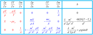
Figure 1. The matrix of Partial derivative coefficients.

The partial derivatives with respect to time and space are denoted as matrix A and B, respectively, and matrix C is the right-hand term of Eqs. (14-16).

A = (\begin{matrix} \frac{ρY}{p} & - \frac{ρX}{T} & 0 \\ X & - ρ c_{p} & 0 \\ 0 & 0 & \frac{1}{A} \end{matrix}) B = (\begin{matrix} 0 & 0 & \frac{1}{A} \\ \frac{mX}{ρA} & - \frac{m c_{p}}{ρA} & 0 \\ 1 - \frac{m^{2}}{ρ^{2} A^{2}} \frac{ρY}{p} & \frac{m^{2}}{ρ^{2} A^{2}} \frac{ρX}{T} & \frac{2 m}{ρ A^{2}} \end{matrix})

C = {(\begin{matrix} 0 & \frac{λ}{d} \frac{m^{3}}{2 ρ^{2} A^{3}} - \frac{4 KD (T - T_{0})}{d^{2}} & \frac{λ}{d} \frac{m^{2}}{2 ρ A^{2}} + ρg ∙ \sin θ \end{matrix})}^{T}

Calculate the eigenvalues of the matrix

{(A^{- 1} B)}^{T}

ω_{1} = \frac{m}{ρA}

ω_{2} = \frac{m}{ρA} + a

ω_{3} = \frac{m}{ρA} - a

where a is the gas sonic velocity,

a = {(\frac{ρY}{p} - \frac{X^{2}}{c_{p} T})}^{- \frac{1}{2}}

, m/s.

Calculate the eigenvectors of matrix

{(A^{- 1} B)}^{T}

as the combination coefficients of Eqs. (14-16).

ϖ_{1} = {(\begin{matrix} 0 & 1 & 0 \end{matrix})}^{T}

ϖ_{2} = {(\begin{matrix} a - \frac{m}{ρA} & - \frac{aX}{c_{p} T} & 1 \end{matrix})}^{T}

ϖ_{3} = {(\begin{matrix} a + \frac{m}{ρA} & - \frac{aX}{c_{p} T} & - 1 \end{matrix})}^{T}

Based on the eigenvalues ω₁, ω₂, ω₃ and the combination coefficients ϖ₁, ϖ₂, ϖ₃, the Eqs. (14-16) are converted into ODEs along the characteristic lines, i.e. characteristic equations:

1) Left characteristic equation

\{\begin{matrix} ω = \frac{dx}{dτ} = \frac{m}{ρA} + a \\ (1 - \frac{ma}{ρA} \cdot \frac{ρY}{p}) \frac{dp}{dτ} + \frac{ma}{ρA} \cdot \frac{ρX}{T} \cdot \frac{dT}{dτ} + \frac{a}{A} \cdot \frac{dm}{dτ} \\ = \frac{a^{2} X}{c_{p} T} [\frac{λ}{d} \cdot \frac{m^{3}}{2 ρ^{2} A^{3}} - \frac{4 KD (T - T_{0})}{d^{2}}] - ρa (\frac{λ}{d} \cdot \frac{m^{2}}{ρ^{2} A^{2}} + g ∙ \sin θ) \end{matrix}

(17)

2) Right characteristic equation

\{\begin{matrix} ω = \frac{dx}{dτ} = \frac{m}{ρA} - a \\ (1 + \frac{ma}{ρA} \cdot \frac{ρY}{p}) \frac{dp}{dτ} - \frac{ma}{ρA} \cdot \frac{ρX}{T} \cdot \frac{dT}{dτ} - \frac{a}{A} \cdot \frac{dm}{dτ} \\ = \frac{a^{2} X}{c_{p} T} [\frac{λ}{d} \cdot \frac{m^{3}}{2 ρ^{2} A^{3}} - \frac{4 KD (T - T_{0})}{d^{2}}] + ρa (\frac{λ}{d} \cdot \frac{m^{2}}{ρ^{2} A^{2}} + g ∙ \sin θ) \end{matrix}

(18)

3) Middle characteristic equation

\{\begin{matrix} ω = \frac{dx}{dτ} = \frac{m}{ρA} \\ X \frac{dp}{dτ} - ρ c_{p} \frac{dT}{dτ} = \frac{4 KD (T - T_{0})}{d^{2}} - \frac{λ}{d} \frac{m^{3}}{2 ρ^{2} A^{3}} \end{matrix}

(19)

3.3. Discretization and Solution

3.3.1. Discretization

As the characteristic line, the gas flow rate and the gas sonic velocity cannot be expressed explicitly in terms of the time variable τ and spatial variable x; it is almost impossible to solve the characteristic equations directly by the integral method. This section uses the explicit characteristic difference method combined with rectangular grids to determine the numerical solution, as shown in Figure 2.

Download: Download full-size image

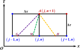
Figure 2. Explicit characteristic difference grid.

Discretizing the Eqs. (17-19) on the Explicit characteristic difference grids, as shown in Figure 2, we can obtain the finite difference equations (20-22) as follows:

1) Left − AG

⟨A⟩ \cdot Δ p^{+} + ⟨B⟩ \cdot Δ T^{+} + ⟨C⟩ \cdot Δ m^{+} = ⟨D⟩ \cdot Δ τ

(20)

2) Right − AH

⟨E⟩ \cdot Δ p^{-} - ⟨B⟩ \cdot Δ T^{-} - ⟨C⟩ \cdot Δ m^{-} = ⟨F⟩ \cdot Δ τ

(21)

3) Middle − AM

⟨G⟩ \cdot Δ p^{0} - ⟨H⟩ \cdot Δ T^{0} = ⟨K⟩ \cdot Δ τ

(22)

where the symbol

⟨⟩

indicates the average value along the characteristic line AG, AH, or AM.

⟨A⟩ = 1 - \frac{ma}{A} \cdot \frac{Y}{p}

⟨B⟩ = \frac{ma}{A} \cdot \frac{X}{T}

⟨C⟩ = \frac{a}{A}

⟨D⟩ = \frac{a^{2} X}{c_{p} T} [\frac{λ}{d} \cdot \frac{m^{3}}{2 ρ^{2} A^{3}} - \frac{4 KD (T - T_{0})}{d^{2}}] - ρa (\frac{λ}{d} \cdot \frac{m^{2}}{ρ^{2} A^{2}} + g ∙ \sin θ)

⟨E⟩ = 1 + \frac{ma}{A} \cdot \frac{Y}{p}

⟨F⟩ = \frac{ma}{A} \cdot \frac{X}{T}

⟨G⟩ = \frac{a}{A}

⟨H⟩ = \frac{a^{2} X}{c_{p} T} [\frac{λ}{d} \cdot \frac{m^{3}}{2 ρ^{2} A^{3}} - \frac{4 KD (T - T_{0})}{d^{2}}] + ρa (\frac{λ}{d} \cdot \frac{m^{2}}{ρ^{2} A^{2}} + g ∙ \sin θ)

⟨K⟩ = X

⟨M⟩ = ρ c_{p}

⟨N⟩ = \frac{4 KD (T - T_{0})}{d^{2}} - \frac{λ}{d} \frac{m^{3}}{2 ρ^{2} A^{3}}

3.3.2. Inner Node and Boundary Conditions

The solution of the finite characteristic difference Eqs. (20-22) varies depending on the location of the mesh nodes. Along the direction of the gas flow of the gas pipeline, the upstream and downstream boundaries are noted as the left and right boundaries, respectively. The nodes can thus be divided into three categories: inner nodes and left and right boundary nodes, which are discussed below.

1) Inner nodes

As shown in Figure 2, node A is the inner node to be determined. Since the intersection nodes of the characteristic lines and the difference grids are not exactly located on the nodes, the interpolation factor

η ∙Δ τ / Δ x

is needed to calculate the flow parameters of

ϕ_{G}

ϕ_{H}

and

ϕ_{M}

, where

ϕ

denotes the flow parameters, such as pressure p, temperature T, or mass flow rate m.

Eqs. (23-25) can calculate the interpolation factor.

η_{+} = \frac{1}{2} [(a_{G} + w_{G}) + (a_{j}^{n + 1} + w_{j}^{n + 1})]

(23)

η_{-} = \frac{1}{2} [(a_{H} - w_{H}) + (a_{j}^{n + 1} - w_{j}^{n + 1})]

(24)

η_{0} = \frac{1}{2} (w_{M} + w_{j}^{n + 1})

(25)

Initial iteration value of Eqs. (23-25):

η_{+}^{[0]} = \frac{1}{2} [(a_{j - 1}^{n} + w_{j - 1}^{n}) + (a_{j}^{n} + w_{j}^{n})]

η_{-}^{[0]} = \frac{1}{2} [(a_{j + 1}^{n} - w_{j + 1}^{n}) + (a_{j}^{n} - w_{j}^{n})]

η_{0}^{[0]} = \frac{1}{2} (w_{j - 1}^{n} + w_{j}^{n})

Hence, the flow parameters of the intersection nodes can be obtained through linear interpolation.

ϕ_{G} = \frac{η_{+} \cdot Δ τ}{Δ x} ϕ_{j - 1}^{n} + (1 - \frac{η_{+} \cdot Δ τ}{Δ x}) ϕ_{j}^{n}

(26)

ϕ_{H} = \frac{η_{-} \cdot Δ τ}{Δ x} ϕ_{j + 1}^{n} + (1 - \frac{η_{-} \cdot Δ τ}{Δ x}) ϕ_{j}^{n}

(27)

ϕ_{M} = \frac{η_{0} \cdot Δ τ}{Δ x} ϕ_{j - 1}^{n} + (1 - \frac{η_{0} \cdot Δ τ}{Δ x}) ϕ_{j}^{n}

(28)

The average values of Ψ, where Ψ denotes the characteristic equation coefficients or right-hand side terms, were calculated from the interpolated flow parameters

ϕ_{G}

ϕ_{H}

and

ϕ_{M}

, as listed below:

{⟨Ψ⟩}_{+} = \frac{1}{2} (Ψ_{G} + Ψ_{j}^{n + 1})

(29)

{⟨Ψ⟩}_{-} = \frac{1}{2} (Ψ_{H} + Ψ_{j}^{n + 1})

(30)

{⟨Ψ⟩}_{0} = \frac{1}{2} (Ψ_{M} + Ψ_{j}^{n + 1})

(31)

The linear algebraic equations for the flow parameters of node A as described in Eq. (32):

(\begin{matrix} ⟨A⟩ & ⟨B⟩ & ⟨C⟩ \\ ⟨E⟩ & - ⟨F⟩ & - ⟨G⟩ \\ ⟨K⟩ & - ⟨M⟩ & 0 \end{matrix}) (\begin{matrix} p_{j}^{n + 1} \\ T_{j}^{n + 1} \\ m_{j}^{n + 1} \end{matrix}) = (\begin{matrix} ⟨A⟩ \cdot p_{G} + ⟨B⟩ \cdot T_{G} + ⟨C⟩ \cdot m_{G} + ⟨D⟩ \cdot Δ τ \\ ⟨E⟩ \cdot p_{H} - ⟨F⟩ \cdot T_{H} - ⟨G⟩ \cdot m_{H} + ⟨H⟩ \cdot Δ τ \\ ⟨K⟩ \cdot p_{M} - ⟨M⟩ \cdot T_{M} + ⟨N⟩ \cdot Δ τ \end{matrix})

(32)

Thus, in solving Eq. (32), the flow parameters of node A are acquired.

2) Left boundary condition

As shown in Figure 3, the left boundary node has only a right characteristic equation. Since there are three basic solution variables to be solved, two additional boundary conditions are needed.

Download: Download full-size image

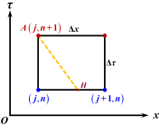
Figure 3. Left boundary condition schematic.

There are three options for the left boundary condition.

(1) Pressure and Temperature

m_{j}^{n + 1} = m_{H} + \frac{[⟨E⟩ (p_{j}^{n + 1} - p_{H}) - ⟨F⟩ (T_{j}^{n + 1} - T_{H}) - ⟨H⟩ ∙ Δ τ]}{⟨G⟩}

(33)

(2) Temperature and mass flow rate

p_{j}^{n + 1} = p_{H} + \frac{[⟨F⟩ (T_{j}^{n + 1} - T_{H}) + ⟨G⟩ (m_{j}^{n + 1} - m_{H}) + ⟨H⟩ ∙ Δ τ]}{⟨E⟩}

(34)

(3) Pressure and mass flow rate

T_{j}^{n + 1} = T_{H} + \frac{[⟨E⟩ (p_{j}^{n + 1} - p_{H}) - ⟨G⟩ (m_{j}^{n + 1} - m_{H}) - ⟨H⟩ ∙ Δ τ]}{⟨F⟩}

(35)

3) Right boundary condition

Download: Download full-size image

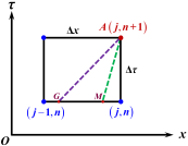
Figure 4. Right boundary condition schematic.

As shown in Figure 4, the right boundary node has two characteristic equations, and there are three essential solution variables to be solved, so one additional boundary condition is needed.

There are also three options for the right boundary condition.

(1) Temperature

\{\begin{matrix} p_{j}^{n + 1} = p_{M} + \frac{[⟨M⟩ (T_{j}^{n + 1} - T_{M}) + ⟨N⟩ ∙ Δ τ]}{⟨K⟩} \\ m_{j}^{n + 1} = m_{G} + \frac{[⟨D⟩ ∙ Δ τ - ⟨A⟩ (p_{j}^{n + 1} - p_{G}) - ⟨B⟩ (T_{j}^{n + 1} - T_{G})]}{⟨C⟩} \end{matrix}

(36)

(2) Pressure

\{\begin{matrix} T_{j}^{n + 1} = T_{M} + \frac{[⟨K⟩ (p_{j}^{n + 1} - p_{M}) - ⟨N⟩ ∙ Δ τ]}{⟨M⟩} \\ m_{j}^{n + 1} = m_{G} + \frac{[⟨D⟩ ∙ Δ τ - ⟨A⟩ (p_{j}^{n + 1} - p_{G}) - ⟨B⟩ (T_{j}^{n + 1} - T_{G})]}{⟨C⟩} \end{matrix}

(37)

(3) Mass flow rate

\{\begin{matrix} p_{j}^{n + 1} = \frac{[\begin{matrix} (⟨B⟩ ⟨N⟩ + ⟨D⟩ ⟨M⟩) ∙ Δ τ - ⟨C⟩ ⟨M⟩ (m_{j}^{n + 1} - m_{G}) + \\ ⟨B⟩ ⟨K⟩ p_{M} + ⟨A⟩ ⟨M⟩ p_{G} + ⟨B⟩ ⟨M⟩ (T_{G} - T_{M}) \end{matrix}]}{(⟨B⟩ ⟨K⟩ + ⟨A⟩ ⟨M⟩)} \\ T_{j}^{n + 1} = T_{M} + \frac{[⟨K⟩ (p_{j}^{n + 1} - p_{M}) - ⟨N⟩ ∙ Δ τ]}{⟨M⟩} \end{matrix}

(38)

Considering the combination of left and right boundaries in the solution process, there are

C_{3}^{2} × C_{3}^{1} =9

combinations of boundary conditions that the MOC can handle.

3.3.3. Initial Condition

The initial condition is the starting condition for the transient simulation of the pipeline segment, which can be determined by the step marching method. As shown in Figure 5, the pipeline is divided into small segments, and then the hydraulic-thermal parameters are calculated sequentially. The temperature and pressure at the starting point are an approximation of the average temperature T_pj and pressure p_pj of the small segment, respectively. The specific calculation procedures are as follows:

Download: Download full-size image

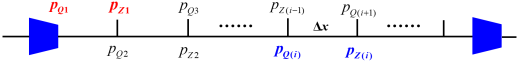
Figure 5. The schematic of the step marching method.

(1) Divide the pipeline into subsections and round up N = CEILING(L/Δx);

(2) i = 1, the temperature and pressure at the beginning of the pipeline are used as T_pj and pressure p_pj, and the physical parameters of gas can be calculated from the EOS. Then the T_i₊₁ and p_i₊₁ of the first subsection is obtained from the hydraulic-thermal calculation.

(3) i = i + 1, let T_pj(i) = T(i−1), p_pj(i) = p(i−1), and then perform step (2) to obtain the T(i) and p(i) of the i-th subsection;

(4) Following the procedure (2) and (3), the temperature and pressure at each node of the pipeline are obtained.

3.3.4. The Continuity Equation on Gas Composition

The conservation of mass for each composition i of the natural gas is expressed independently as the composition continuity equation. On the difference grids shown in Figure 6, the explicit difference scheme is used to discretize the composition continuity equations:

Download: Download full-size image

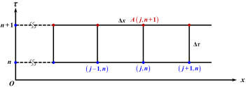
Figure 6. The discretization of the continuity equation on gas composition.

{(c_{i})}_{j}^{n + 1} = {(c_{i})}_{j}^{n} - w_{j}^{n} \cdot \frac{Δ τ}{Δ x} [{(c_{i})}_{j}^{n} - {(c_{i})}_{j - 1}^{n}]

(39)

x_{i} = \frac{c_{i}}{M_{i}} / \sum_{j} (\frac{c_{j}}{M_{j}})

(40)

c_{i} = x_{i} M_{i} / \sum_{j} ({x_{j} M}_{j})

(41)

Where x_i and M_i are the mole fraction and mole mass of the natural gas component i, respectively, from the natural gas mole fraction, the natural gas heating value can be calculated according to GB/T 11062−2020 (ISO 6976:2016 IDT).

3.3.5. Stability Criterion

The stability criterion

[17, 18]

, due to the CFL criterion, is that the domain of dependence on the exact solution is contained within the domain of dependence on the numerical solution, as follows:

Δ τ \leq \min_{1 \leq i \leq N} {(\frac{Δ x}{a + |w|})}_{i}

(42)

3.3.6. Overall Solution Process

Download: Download full-size image

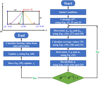
Figure 7. The framework of gas composition tracking based on the MOC.

The detailed calculation procedures for gas composition tracking based on the MOC are as follows:

(1) The coefficients and their right-hand terms of the characteristic difference equations are calculated from the initial conditions;

(2) Solving the characteristic difference Eqs. (20-22) to yield the flow parameters at node A: T, p, and m.

(3) Solve the gas EOS Eq. (4) to obtain the density ρ and update the gas flow rate w, sonic velocity a and other physical parameters;

(4) Determine the composition continuity Eq. (39) and update the natural gas composition;

(5) The coefficients of the characteristic difference equations are recalculated using the improved physical parameters.

(6) The improved flow parameters are the initial values for the following iterative computation.

(7) Repeat the step (2-6) until a converged solution is obtained.

The framework of gas composition tracking based on the MOC is shown in Figure 7.

4. Case Study

In this section, one case will be presented to show the performance of the proposed method.

A pipeline segment is 280 km in length. The outer and inner diameter of the gas pipeline are 1016 mm and 981.2 mm, respectively. The equivalent roughness of the inner pipe wall is the 10 μm. The pipeline upstream pressure is 10 MPa, and the annual transmission capacity of the pipeline is 120×10⁸ m³. The section of the pipeline transmission efficiency is 0.95, and the upstream temperature is 55 °C. The average overall heat transfer coefficient of the pipeline is 2.16 W/(m²·K), and the natural ground temperature of soil in buried depth is 12 °C. The dynamic viscosity of the gas is 1.10125×10⁻⁹ Pa·s, and the upstream gas composition is shown in Table 1.

Table 1. Upstream gas composition.

Composition	mole fraction %
CH₄	97.739	95.126	92.302	88.243
N₂	0.7022	0.6928	0.6843	0.7046
CO₂	1.1131	1.1541	1.2140	1.3081
C₂	0.401	2.991	2.7428	6.124
C₃	0.0405	0.0322	3.0531	3.6172
iC₄	0.0012	0.0013	0.0014	0.0011
nC₄	0.0021	0.0015	0.0014	0.0013
iC5	0.0002	0.0004	0.0003	0.0002
nC5	0.0005	0.0004	0.0004	0.0003
nC6	0.0002	0.0003	0.0003	0.0002

The downstream boundary condition can be determined by the hourly asymmetry coefficient, as shown in Figure 8.

Download: Download full-size image

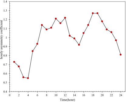
Figure 8. The hourly asymmetry coefficient versus time.

Download: Download full-size image

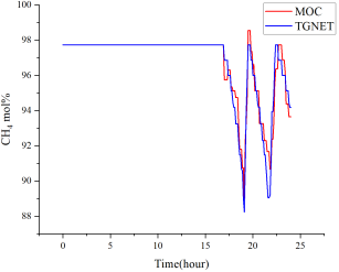
Figure 9. The mole fraction of CH₄ versus time.

Download: Download full-size image

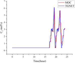
Figure 10. The mole fraction of C₂H₆ versus time.

Download: Download full-size image

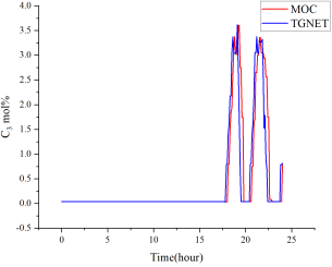
Figure 11. The mole fraction of C₃H₈ versus time.

Based on a natural gas pipeline segment as an example, a transient simulation model for the tracking of natural gas composition is established using the MOC. Set the time-dependent data of natural gas components as the boundary condition of the pipeline upstream. After 24 hours of operation, the results, which are calculated by the MOC and compared with the commercial simulation software Pipeline Studio for Gas (TGNET)

[19]

, are shown in Figure 9, Figure 10 and Figure 11.

Figure 9, Figure 10 and Figure 11 show the variation of the mole fraction of CH₄, C₂ and C₃ downstream of the pipeline, respectively. In this case, the results show that the impact on gas composition changes the upstream of the pipeline, which needs about 16 hours to affect the downstream. The average absolute deviations between the MOC and TGNET of the CH₄, C₂ and C₃ mole fractions are 0.897%, 0.657% and 0.508%, respectively, all less than 1%. Hence, the MOC exhibits a comparable computational accuracy performance to TGNET.

5. Conclusions and Recommendations

This article presents how natural gas composition tracking can be achieved for the transient gas pipeline based on the MOC. The main conclusions are as follows:

(1) According to the case study, the proposed method can track gas composition, and the average absolute deviations are within 1% compared with TGNET.

(2) Nine combinations of boundary conditions are derived, which expands the range of application of the origin MOC.

(3) The MOC can meet the demand for actual energy determination requirements at Class B and C metering stations.

(4) It could also provide a theoretical foundation for the homemade gas pipeline simulation software, which tracks gas composition.

In the future, the diversification of gas sources, such as unconventional gas, LNG, and H₂ or biomethane injection, will make the gas composition tracking issues more significant. Herein we have the following recommendations:

(1) The non-pipe elements in the natural gas pipeline system, such as compressors and valves, still need to be taken into account.

(2) Parallel computing techniques can be employed to improve computational efficiency and accelerate convergence.

(3) To attenuate the constraints of the CFL criterion on the time step and knot spacing, the implicit central difference method (ICDM)

[20]

can be applied in regions where the gas composition has little change, while the MOC is adopted in regions where the natural gas composition changes dramatically.

(4) Tracking the gas composition of pipeline networks with hydrogen injection is becoming increasingly essential because hydrogen is recognized worldwide as a cleaner energy source than fossil fuels.

(5) More exact EOS, such as AGA8-92DC and GERG-2008, can be utilized to calculate the thermophysical properties accurately.

Abbreviations

PDEs	Partial Differential Equations
MOC	Method Of Characteristics
CFL	Courant-Friedrichs-Lewy
EOS	Equation of State
ICDM	Implicit Central Difference Method

Acknowledgments

The work is supported by the National Natural Science Foundation of China (Grant No. 52174064). The authors are also thankful to all the reviewers for their insights and constructive comments.

Author Contributions

Da Qi: Conceptualization, Methodology, Software, Writing Original Draft

Changchun Wu: Supervision, Resources, Funding acquisition

Zhe Liu: Supervision, Resources, Review and Editing

Lili Zuo: Supervision, Resources, Funding acquisition

Funding

The work is supported by the National Natural Science Foundation of China (Grant No. 52174064).

Data Availability Statement

The data is available from the corresponding author upon reasonable request.

Conflicts of Interest

The authors declare no conflicts of interest.

References

[1]	Wei C, Tianbo Y, Changwu L, Likai H, Fubing B, Jinchun, N. Advancements in the Natural Gas Measurement System Under a Multi-Source Scenario: A Domestic and International Perspective [J]. Metrology Science and Technology, 2024, 68(1): 3-9, 75. https://doi.org/10.12338/j.issn.2096-9015.2023.0321
[2]	Guandalini G, Colbertaldo P, Campanari S. Dynamic modeling of natural gas quality within transport pipelines in presence of hydrogen injections. Applied Energy. 2017, 185: 1712-1723. https://doi.org/10.1016/j.apenergy.2016.03.006
[3]	Guandalini G, Colbertaldo P, Campanari S. Dynamic Quality Tracking of Natural Gas and Hydrogen Mixture in a Portion of Natural Gas Grid. Energy Procedia. 2015, 75: 1037-1043. https://doi.org/10.1016/j.egypro.2015.07.376
[4]	Chaczykowski M, Zarodkiewicz P. Simulation of natural gas quality distribution for pipeline systems. Energy. 2017, 134: 681-698. https://doi.org/10.1016/j.energy.2017.06.020
[5]	Chaczykowski M, Sund F, Zarodkiewicz P, et al. Gas composition tracking in transient pipeline flow. Journal of Natural Gas Science and Engineering. 2018, 55: 321-330. https://doi.org/10.1016/j.jngse.2018.03.014
[6]	Osiadacz A J, Chaczykowski M. Modeling and Simulation of Gas Distribution Networks in a Multi-energy System Environment. Proceedings of the IEEE. 2020, 108(9): 1580-1595. https://doi.org/10.1109/JPROC.2020.2989114
[7]	Fan D, Gong J, Zhang S, et al. A transient composition tracking method for natural gas pipe networks. Energy. 2021, 215: 119131. https://doi.org/10.1016/j.energy.2020.119131
[8]	Fan D, Study on Transient Simulation and Composition Tracking in Natural Gas Condensate Pipeline Network. Doctoral Dissertation. China University of China, Beijing. 2021, pp. 75-83. https://doi.org/10.27643/d.cnki.gsybu.2021.000196
[9]	Urh, M, Pantoš, M. Gas composition tracking feasibility using transient finite difference θ-scheme model for binary gas mixtures. International Journal of Hydrogen Energy, 2024, 49, 1319-1331. https://doi.org/10.1016/j.ijhydene.2023.11.031
[10]	Bermúdez, A, Shabani, M. Numerical simulation of gas composition tracking in a gas transportation network. Energy, 2022, 247, 123459. https://doi.org/10.1016/j.energy.2022.123459
[11]	Bermúdez, A, Shabani, M. Finite element solution of isothermal gas flow in a network. Journal of Computational Physics, 2019, 396, 616-652. https://doi.org/10.1016/j.jcp.2019.06.063
[12]	Behbahani-Nejad, M, Bermúdez, A, Shabani, M. Finite element solution of a new formulation for gas flow in a pipe with source terms. Journal of Natural Gas Science and Engineering, 2019, 61, 237-250. https://doi.org/10.1016/j.jngse.2018.11.019
[13]	Zihang Z, Saedi, I, Mhanna, S, Wu, K, Mancarella, P. Modelling of gas network transient flows with multiple hydrogen injections and gas composition tracking. International Journal of Hydrogen Energy, 2022, 47(4), 2220-2233. https://doi.org/10.1016/j.ijhydene.2021.10.165
[14]	Wang, C, Zhou, D, Xiao, W, Shui, C, Ma, T, Chen, P, Yan, J. Research on the dynamic characteristics of natural gas pipeline network with hydrogen injection considering line-pack influence. International Journal of Hydrogen Energy, 2023, 48(65), 25469-25486. https://doi.org/10.1016/j.ijhydene.2023.03.298
[15]	Mohitpour, M, Golshan, H, Murray, A. Pipeline Design & Construction: A Practical Approach, Third Edition. ASME Press, 2007, pp. 263-268. https://doi.org/10.1115/1.802574
[16]	Starling K E. Fluid Thermodynamic Properties for Light Petroleum Systems. Houston: Gulf Publishing Company. 1973, pp. 1-3, 220-223. https://searchworks.stanford.edu/view/925749
[17]	Gnedin, N. Y., Semenov, V. A., Kravtsov, A. V. Enforcing the Courant–Friedrichs–Lewy condition in explicitly conservative local time stepping schemes. Journal of Computational Physics, 2018, 359, 93-105. https://doi.org/10.1016/j.jcp.2018.01.008
[18]	Thorley, A. R. D., Tiley, C. H. Unsteady and transient flow of compressible fluids in pipelines—A review of theoretical and some experimental studies. International journal of heat and fluid flow, 1987, 8(1), 3-15. https://doi.org/10.1016/0142-727X(87)90044-0
[19]	Weihe H, Honggang C, et al. Energy measurement method of annular pipeline network with multi-gas sources based on operation simulation. Chemical Engineering of Oil & Gas, 2022, 51(5): 117-123. https://doi.org/10.3969/j.issn.1007-3426.2022.5.018
[20]	Qian C, Aocheng G, Feng C, F, et al. A transient gas pipeline network simulation model for decoupling the hydraulic-thermal process and the component tracking process. Energy, 2024, 131613. https://doi.org/10.1016/j.energy.2024.131613

Cite This Article

Plain Text BibTeX RIS

APA Style

Qi, D., Wu, C., Liu, Z., Zuo, L. (2024). Gas Composition Tracking in a Transient Pipeline Using the Method of Characteristics. American Journal of Energy Engineering, 12(2), 32-42. https://doi.org/10.11648/j.ajee.20241202.12

Copy | Download

ACS Style

Qi, D.; Wu, C.; Liu, Z.; Zuo, L. Gas Composition Tracking in a Transient Pipeline Using the Method of Characteristics. Am. J. Energy Eng. 2024, 12(2), 32-42. doi: 10.11648/j.ajee.20241202.12

Copy | Download

AMA Style

Qi D, Wu C, Liu Z, Zuo L. Gas Composition Tracking in a Transient Pipeline Using the Method of Characteristics. Am J Energy Eng. 2024;12(2):32-42. doi: 10.11648/j.ajee.20241202.12

Copy | Download

@article{10.11648/j.ajee.20241202.12,
  author = {Da Qi and Changchun Wu and Zhe Liu and Lili Zuo},
  title = {Gas Composition Tracking in a Transient Pipeline Using the Method of Characteristics
},
  journal = {American Journal of Energy Engineering},
  volume = {12},
  number = {2},
  pages = {32-42},
  doi = {10.11648/j.ajee.20241202.12},
  url = {https://doi.org/10.11648/j.ajee.20241202.12},
  eprint = {https://article.sciencepublishinggroup.com/pdf/10.11648.j.ajee.20241202.12},
  abstract = {For a gas pipeline with multiple gas sources, the significance of tracking the composition of natural gas is increasing with the implementation of X+1+X system for the natural gas industry in China. Mathematically, the tracking problem is usually described by a system of partial differential equations (PDEs). The continuity equation on gas composition has been developed to track natural gas composition according to the law of mass conservation. The algorithm resulting from the method of characteristics (MOC) is proposed to solve the system of PDEs. Compared to the original MOC, numerical solutions of the continuity equation on gas composition are obtained after the hydraulic calculation and thermal calculation. Moreover, different combinations of boundary conditions for the MOC are derived, which could expand the range of application of the MOC and be applicable to various operating conditions. The heating values of diverse gas sources have been determined following the methods documented in ISO 6976:2016. The case study of a gas pipeline in China verified the validity of the algorithm via the commercial simulation software Pipeline Studio for Gas (TGNET). The heating value and gas composition obtained by the algorithm can be used in the custody transfer metering of natural gas pipelines for Class B and C metering stations described in GB/T 18603−2014.
},
 year = {2024}
}

Copy | Download

TY  - JOUR
T1  - Gas Composition Tracking in a Transient Pipeline Using the Method of Characteristics

AU  - Da Qi
AU  - Changchun Wu
AU  - Zhe Liu
AU  - Lili Zuo
Y1  - 2024/06/19
PY  - 2024
N1  - https://doi.org/10.11648/j.ajee.20241202.12
DO  - 10.11648/j.ajee.20241202.12
T2  - American Journal of Energy Engineering
JF  - American Journal of Energy Engineering
JO  - American Journal of Energy Engineering
SP  - 32
EP  - 42
PB  - Science Publishing Group
SN  - 2329-163X
UR  - https://doi.org/10.11648/j.ajee.20241202.12
AB  - For a gas pipeline with multiple gas sources, the significance of tracking the composition of natural gas is increasing with the implementation of X+1+X system for the natural gas industry in China. Mathematically, the tracking problem is usually described by a system of partial differential equations (PDEs). The continuity equation on gas composition has been developed to track natural gas composition according to the law of mass conservation. The algorithm resulting from the method of characteristics (MOC) is proposed to solve the system of PDEs. Compared to the original MOC, numerical solutions of the continuity equation on gas composition are obtained after the hydraulic calculation and thermal calculation. Moreover, different combinations of boundary conditions for the MOC are derived, which could expand the range of application of the MOC and be applicable to various operating conditions. The heating values of diverse gas sources have been determined following the methods documented in ISO 6976:2016. The case study of a gas pipeline in China verified the validity of the algorithm via the commercial simulation software Pipeline Studio for Gas (TGNET). The heating value and gas composition obtained by the algorithm can be used in the custody transfer metering of natural gas pipelines for Class B and C metering stations described in GB/T 18603−2014.

VL  - 12
IS  - 2
ER  -

Copy | Download

Author Information

Da Qi

National Engineering Laboratory of Pipeline Safety, Beijing Key Laboratory of Urban Oil and Gas Distribution Technology, China University of Petroleum-Beijing, Beijing, China

Biography: Da Qi is a doctoral candidate. His supervisors are Professor Changchun Wu and Professor Lili Zuo. He received his Bachelor's degree in Oil and gas Storage and Transportation from China University of Petroleum, Beijing, in 2005. His research interests include the operation simulation (Energy determination) of natural gas networks.

Research Fields: Operation simulation (energy determination) of natural gas networks.

Contact Email

http://orcid.org/0009-0002-3426-9529
Changchun Wu

National Engineering Laboratory of Pipeline Safety, Beijing Key Laboratory of Urban Oil and Gas Distribution Technology, China University of Petroleum-Beijing, Beijing, China

Biography: Changchun Wu is a professor at the China University of Petroleum, Beijing, College of Mechanical and Transportation Engineering. He received his Master's degree in Oil and gas Storage and Transportation from the Beijing Graduate Department of East China Petroleum Institute in 1985. His research interests cover operation simulation, design and operation optimization, and reliability assessment of oil and gas networks. He is a member of the Chinese Petroleum Society.

Research Fields: Operation simulation, design and operation optimization, reliability assessment of oil and gas network.

Contact Email

http://orcid.org/0009-0001-6704-7044
Zhe Liu

Nanjing Metrology Research Center of West-East Gas Pipeline Company, Nanjing, China

Biography: Zhe Liu is a senior engineer at Nanjing Metrology Research Centre PipeChina West-East Gas Pipeline Company. She received her Master's degree in Measuring and Testing Technologies and Instruments from China Jiliang University in 2013. Her research interests include natural gas metering technology. She has published 20 papers, authorized six invention patents, and been awarded five scientific and technological awards.

Research Fields: Natural gas metering technology and fluid stability.

Contact Email

http://orcid.org/0009-0007-6279-7659
Lili Zuo

National Engineering Laboratory of Pipeline Safety, Beijing Key Laboratory of Urban Oil and Gas Distribution Technology, China University of Petroleum-Beijing, Beijing, China

Biography: Lili Zuo is a professor at the China University of Petroleum, Beijing, College of Mechanical and Transportation Engineering. She acquired her Master's and PhD degree in Oil and Gas Storage and Transportation from China University of Petroleum, Beijing, in 2005 and 2008, respectively. Her research interests cover operation simulation and optimization and engineering economics of oil and gas pipelines.

Research Fields: Operation simulation and optimization, engineering economics of oil and gas pipelines.

Contact Email

http://orcid.org/0000-0002-3272-5124

Download PDF

Submit an Article

Table 1

Table 1. Upstream gas composition.

Plain Text BibTeX RIS

APA Style

Qi, D., Wu, C., Liu, Z., Zuo, L. (2024). Gas Composition Tracking in a Transient Pipeline Using the Method of Characteristics. American Journal of Energy Engineering, 12(2), 32-42. https://doi.org/10.11648/j.ajee.20241202.12

Copy | Download

ACS Style

Qi, D.; Wu, C.; Liu, Z.; Zuo, L. Gas Composition Tracking in a Transient Pipeline Using the Method of Characteristics. Am. J. Energy Eng. 2024, 12(2), 32-42. doi: 10.11648/j.ajee.20241202.12

Copy | Download

AMA Style

Qi D, Wu C, Liu Z, Zuo L. Gas Composition Tracking in a Transient Pipeline Using the Method of Characteristics. Am J Energy Eng. 2024;12(2):32-42. doi: 10.11648/j.ajee.20241202.12

Copy | Download

@article{10.11648/j.ajee.20241202.12,
  author = {Da Qi and Changchun Wu and Zhe Liu and Lili Zuo},
  title = {Gas Composition Tracking in a Transient Pipeline Using the Method of Characteristics
},
  journal = {American Journal of Energy Engineering},
  volume = {12},
  number = {2},
  pages = {32-42},
  doi = {10.11648/j.ajee.20241202.12},
  url = {https://doi.org/10.11648/j.ajee.20241202.12},
  eprint = {https://article.sciencepublishinggroup.com/pdf/10.11648.j.ajee.20241202.12},
  abstract = {For a gas pipeline with multiple gas sources, the significance of tracking the composition of natural gas is increasing with the implementation of X+1+X system for the natural gas industry in China. Mathematically, the tracking problem is usually described by a system of partial differential equations (PDEs). The continuity equation on gas composition has been developed to track natural gas composition according to the law of mass conservation. The algorithm resulting from the method of characteristics (MOC) is proposed to solve the system of PDEs. Compared to the original MOC, numerical solutions of the continuity equation on gas composition are obtained after the hydraulic calculation and thermal calculation. Moreover, different combinations of boundary conditions for the MOC are derived, which could expand the range of application of the MOC and be applicable to various operating conditions. The heating values of diverse gas sources have been determined following the methods documented in ISO 6976:2016. The case study of a gas pipeline in China verified the validity of the algorithm via the commercial simulation software Pipeline Studio for Gas (TGNET). The heating value and gas composition obtained by the algorithm can be used in the custody transfer metering of natural gas pipelines for Class B and C metering stations described in GB/T 18603−2014.
},
 year = {2024}
}

Copy | Download

TY  - JOUR
T1  - Gas Composition Tracking in a Transient Pipeline Using the Method of Characteristics

AU  - Da Qi
AU  - Changchun Wu
AU  - Zhe Liu
AU  - Lili Zuo
Y1  - 2024/06/19
PY  - 2024
N1  - https://doi.org/10.11648/j.ajee.20241202.12
DO  - 10.11648/j.ajee.20241202.12
T2  - American Journal of Energy Engineering
JF  - American Journal of Energy Engineering
JO  - American Journal of Energy Engineering
SP  - 32
EP  - 42
PB  - Science Publishing Group
SN  - 2329-163X
UR  - https://doi.org/10.11648/j.ajee.20241202.12
AB  - For a gas pipeline with multiple gas sources, the significance of tracking the composition of natural gas is increasing with the implementation of X+1+X system for the natural gas industry in China. Mathematically, the tracking problem is usually described by a system of partial differential equations (PDEs). The continuity equation on gas composition has been developed to track natural gas composition according to the law of mass conservation. The algorithm resulting from the method of characteristics (MOC) is proposed to solve the system of PDEs. Compared to the original MOC, numerical solutions of the continuity equation on gas composition are obtained after the hydraulic calculation and thermal calculation. Moreover, different combinations of boundary conditions for the MOC are derived, which could expand the range of application of the MOC and be applicable to various operating conditions. The heating values of diverse gas sources have been determined following the methods documented in ISO 6976:2016. The case study of a gas pipeline in China verified the validity of the algorithm via the commercial simulation software Pipeline Studio for Gas (TGNET). The heating value and gas composition obtained by the algorithm can be used in the custody transfer metering of natural gas pipelines for Class B and C metering stations described in GB/T 18603−2014.

VL  - 12
IS  - 2
ER  -

Copy | Download