The UK Economy and Oil Price Shocks: An Empirical Assessment Under the New Keynesian Framework

Vivek Singh Chauhan

doi:doi:10.11648/j.ijeee.20261103.13

Research Article |

| Peer-Reviewed

The UK Economy and Oil Price Shocks: An Empirical Assessment Under the New Keynesian Framework

Vivek Singh Chauhan^*

Published in International Journal of Economy, Energy and Environment (Volume 11, Issue 3)

Received: 9 February 2026 Accepted: 25 February 2026 Published: 18 June 2026

Views: Downloads:

Download PDF

Share This Article

Twitter
Linked In
Facebook

Abstract

This study investigates the macroeconomic effects of the global oil price shocks on the United Kingdom from 2004 to 2024 within the framework of the New Keynesian (NK) model for small open economies. Employing reduced-form VAR and SVAR approaches, we analyse the dynamic responses of real GDP, inflation, the interest rate, and the real exchange rate to exogenous oil price movements. Beyond interpreting these effects, the study critically assesses how closely real-world outcomes align with NK model predictions. From VAR analysis, our findings (by interpretating impulse-response functions) largely validate the NK framework. For a positive oil price shock, it results in cost-push inflation by raising firms' marginal production costs. Inflation increases persistently in the short to medium term, while output contracts due to declining real income and tighter financial conditions. Monetary policy responds endogenously through interest rate hikes aimed at stabilizing inflation expectations, amplifying short-run output losses. The real exchange rate depreciates following adverse oil shocks, reflecting both deteriorating trade conditions and monetary tightening dynamics. While findings largely validate the NK model's qualitative implications, the study has its own diagnostic limitations such as non-normal residuals and model simplification. Overall, the study provides contribution to empirical evidence validating the relevance of the NK model framework, particularly for understanding oil price shocks to an open small economy.

Published in	International Journal of Economy, Energy and Environment (Volume 11, Issue 3)
DOI	10.11648/j.ijeee.20261103.13
Page(s)	74-96
Creative Commons	This is an Open Access article, distributed under the terms of the Creative Commons Attribution 4.0 International License (http://creativecommons.org/licenses/by/4.0/), which permits unrestricted use, distribution and reproduction in any medium or format, provided the original work is properly cited.
Copyright	Copyright © The Author(s), 2026. Published by Science Publishing Group

Keywords

Macroeconomics, Monetary Economics, New Keynesian Model, Open Economy Setting, UK Economy, Oil Price, VAR, SVAR

1. Introduction and Motivation

Oil price shocks have long been recognised as major drivers of macroeconomic fluctuations worldwide. For an open economy like the UK, these shocks quickly transmit through trade balances, inflation pressures, and financial markets, posing significant challenges for policymakers. While theory provides clear predictions, it remains uncertain how well these models capture real-world dynamics. This essay examines the macroeconomic effects of oil price shocks on the UK economy from 2004 to 2024, using the NK model for small open economies as a theoretical framework. Through a VAR-based framework, we analyse the dynamic responses of real GDP, inflation, interest, and real exchange rate to exogenous oil price movements. Our ultimate aim is to assess whether the real-world dynamics align with the predictions of the NK model, thereby evaluating its empirical validity.

The motivation behind this study is to critically assess the applicability of the NK model in capturing the real-world transmission of external supply shocks. While the model is widely used as a foundation for policy analysis, its predictive power, particularly under external shocks in open economies, remains a subject of ongoing debate. Focusing on oil shocks—a classic and persistent external disturbance—this study provides an opportunity to examine the robustness of the framework in a real-world context. Specifically, it evaluates whether the model’s key mechanisms, such as cost-push inflation and output contraction, manifest in the UK's open economy setting during a period marked by significant global oil price fluctuations.

The structure of the essay is as follows. Section 2 provides historical background on UK and oil prices with graphical analysis. Section 3 constitutes the literature review, outlining the NK model's theoretical foundations and empirical literature on the UK economy and oil prices. Section 4 discusses data and summary statistics, followed by empirical methodology of the VAR-based framework. Section 5 presents the empirical results and findings, focusing on reduced-form VAR and SVAR-IRFs, supported by robust discussion of the framework. Section 6 discusses the findings in light to the NK model’s theoretical expectations.

2. Background: Setting the Scene

As a globally traded commodity, oil has historically played a central role in shaping macroeconomic performance across countries, including the UK. Fluctuations in oil prices influence critical macroeconomic variables such as GDP and inflation, particularly for oil-importing economies. This section provides historical context on the UK's oil trade position, major oil price shocks between 2004–2024 and provides initial insights on the relationship through a graphical analysis.

2.1. The UK Economy and Its Oil Dependency

Globally, the UK is primarily characterised as an oil consumer rather than a supplier. In 2023, it consumed approximately 61.7 million tonnes of oil, accounting for 1.4% of global oil consumption and ranks as the 16th largest consumer worldwide. Historically, the UK became a net importer of crude oil in 2004, however due to the country’s refining capacity and offshore production, it remained a net exporter of oil products. However, by 2013, rising input costs, declining competitiveness, and declining output eventually made the UK a net importer of oil products. By 2023, net oil imports reached 11.5 million tonnes, with oil accounting for 39% of total energy consumption in the UK, mostly driven by oil as an energy source, fuel for transportation, industrial and domestic needs.

[4, 36, 38]

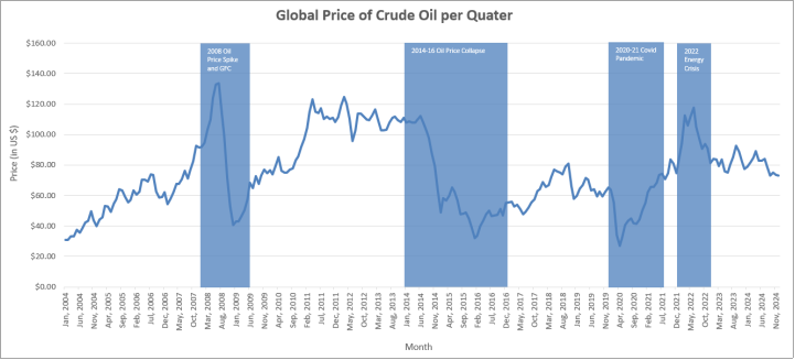
Given its heavy reliance, oil price fluctuations significantly impact the UK economy. Over the study period, we cover four major oil price shocks – 2008 oil spike and GFC, 2014–16 oil price collapse, 2020 COVID-19 crash, and 2022 energy crisis. Table 1 summarises these episodes, with Figure 1 illustrating oil price trends during these events.

Table 1. Four Major Oil Price Shocks

[9]

Event/Shock	Time period	Brief Summary
2008 Oil Price Spike and GFC	2008-09	In mid-2008, oil prices surged to a record high of $147 per barrel due to strong global demand and constrained supply. However, the onset of the GFC in late 2008 led to a sharp decline, with prices plummeting to $40 per barrel by December. The crisis balanced demand and supply, stabilizing prices below $50 per barrel in mid-2009.
2014–2016 Oil Price Collapse	2014-16	In mid-2014, oil prices fell below $50 per barrel, and after a brief recovery, dropped further to $27 per barrel in 2016—the lowest since 2003. This decline resulted from weaker global demand, driven by sluggish economic growth, and increased supply from emerging producers such as Iran.
2020 COVID-19 Pandemic	2020-21	The outbreak of COVID-19 in early 2020 led to worldwide lockdowns, causing a dramatic decline in oil demand. In 2020, prices fell from $65 per barrel in January to $20 per barrel in April—the lowest since 2002. However, a rapid recovery followed, with prices reaching $75 per barrel by June 2021, due to supply constraints as OPEC struggled to keep pace with rebounding demand.
2022 Energy Crisis	2022	In early 2022, Russia’s full-scale invasion of Ukraine and subsequent global sanctions on Russia—the world’s largest oil exporter—triggered a sharp price surge. Oil prices exceeded $100 per barrel, peaking at $127 in March. However, by mid-2022, deteriorating global economic conditions led to a gradual decline, with prices ending the year at approximately $82 per barrel.

Download: Download full-size image

Figure 1. Oil Prices in the UK, with shocks highlighted

[25]

2.2. Preliminary Insight: Oil Prices, GDP, and Inflation Trends

Following the oil prices and key shocks, we conduct a preliminary graphical analysis focusing on the relationship between oil prices and key macroeconomic variables, real GDP and inflation, to providing us initial insights into the influence of oil price fluctuations on UK’s economic performance.

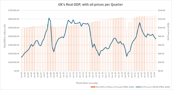
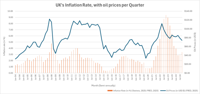
Since 2004, the UK’s real GDP has followed an upward trend, growing at an average annual rate of 1.26% and increased from £499 million in 2004 to £641 million in 2024, primarily driven by rising consumption. Figure 2 suggests a weak relationship between oil prices and real GDP, suggesting that while oil price shocks have an impact, their overall effect on economic growth is limited. Meanwhile, Inflation has increased at an average annual rate of 2.6%, with a sharp spike to nearly 8% in 2022 during the post-pandemic recovery and energy crisis. 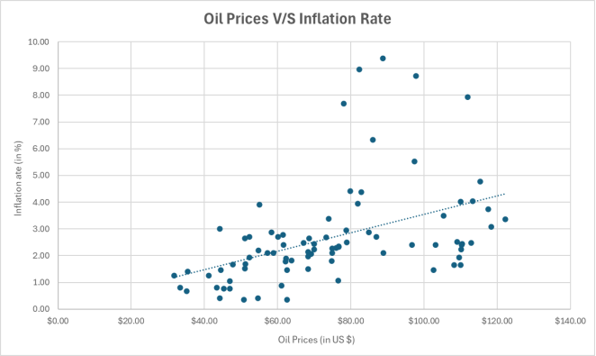Figure 3 suggests a strong relationship between inflation and oil prices, suggesting that oil price fluctuations may constitute as a key driver of inflation in the UK.

[16, 24]

Download: Download full-size image

Figure 2. UK’s Real GDP, with oil prices

[24, 25]

Download: Download full-size image

Figure 3. UK’s Inflation Rate, with oil prices

[16, 25]

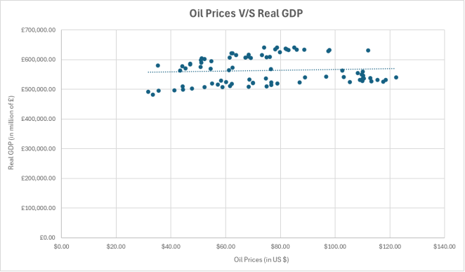
Furthermore, we conduct a scatter plot analysis to verify this correlation trend. Figures 4 and 5 support our initial findings, as the trendline for real GDP exhibits a relatively flat slope, indicating weak correlation with oil prices. Meanwhile, the trendline for inflation demonstrates a steeper slope, reinforcing the strong relationship between oil prices and inflation in the UK.

Download: Download full-size image

Figure 4. Scatter Plot of Real GDP and Oil prices

[24, 25]

Download: Download full-size image

Figure 5. Scatter Plot of Inflation rate and Oil prices

[16, 25]

Summarizing, oil price fluctuations appear to have a relatively modest impact on UK output, but a considerably stronger effect on inflation. These findings provide a preliminary view of the economic impact of oil prices in relationship to the UK’s economy – an oil shock significantly impacts inflation, while GDP remains less sensitive in the short-run. This relationship is further explored in detail in literature review and empirical analysis in the sections that follow.

3. Literature Review: Building the Foundation

This section constitutes a literature review, providing a theoretical and empirical foundation for our study. It establishes the necessary background on the NK model and examines existing literature on the relationship between oil prices and UK’s economy, in need to answer our key research question: ‘How did oil prices affect the UK economy during 2004-2024 under New Keynesian framework?’ The section is structured into two parts. The first half introduces the NK model, covering its historical development, key assumptions, and core mechanisms, along with its limitations. This includes extending the baseline model to SOE. The second half reviews empirical studies on the impact of oil prices on the UK economy, assessing findings from previous established research. Finally, we summarize key insights, identify gaps in the literature, and position our study within this context to address some of these gaps.

3.1. The New Keynesian Model: A Theoretical Perspective

The NK model is a micro-founded DSGE framework incorporating nominal rigidities to explain short-run business cycle fluctuations. The model was developed to analyse how monetary policy interacts with inflation and economic cycles, particularly, how central banks can implement optimal policies to stabilize economic fluctuations. The framework, thus, serves as a relevant tool for policy analysis, demonstrating how interest rate decisions impact asset valuation, investment decisions of economic agents, and ultimately macroeconomic variables like employment, GDP, and inflation.

[22]

The NK model emerged in response to limitations of RBC theory (by Kydland & Prescott), which emphasized technology shocks without incorporating monetary dynamics. Subsequent classical monetary models added a monetary sector but assumed short-run monetary neutrality and the Friedman rule, contradicting the belief in the power of monetary policy to influence real variables such as output and unemployment in short run, supported by empirical research. To address these shortcomings, NK economists introduced nominal rigidities and imperfect competition into the DSGE framework, producing a more realistic depiction of short-run dynamics. Today, the NK model remains a cornerstone of modern macroeconomic research and central bank policymaking.

[22]

The NK model builds on several RBC assumptions such as rational expectations, intertemporal optimization, and consumption smoothing but crucially introduces monetary sectors and policy intervention by allowing nominal rigidities. The model is built on three foundational assumptions: (1) rational expectations and microfoundations, (2) price and wage stickiness, and (3) imperfect competition, thus allowing for monetary policy to influence real economic activity in the short run. The baseline NK model includes three standard shocks: demand shocks affecting households’ consumption and investment decisions (incorporated in NKIS), cost-push shocks arising from unexpected changes in firm’s production costs (incorporated in NKPC) and monetary shocks (reflecting unanticipated policy changes). The paper formalized this model through three core equations: NKIS, NKPC, and monetary policy rule.

[22]

Further models extend the model to a SOE context, incorporating international trade and financial linkages while preserving core nominal rigidities. Unlike the closed-economy version, this model relaxes the assumption of economic agents operating in isolation by allowing them to engage in international trade and foreign financial market under simplifying assumptions such as complete financial markets, the law of one price, and identical preferences, technology, and market structure across countries, thus, creating a framework where it isolates the role monetary policy and exchange rate and shows how external shocks influence domestic inflation and output. This version introduces three additional shocks - exchange-rate shocks, foreign demand shocks, and ToT shocks. The paper formalized this model by deriving modified versions of NKIS curve and NKPC, with additional equation of real exchange rate, ToT.

[22]

Empirical research on the NK model has extensively tested its predictions regarding inflation dynamics, monetary policy transmission, and the effects of shocks on output and inflation. A major focus has been on the NKPC, which posits that inflation depends on expected future inflation and the output gap. However, evidence suggests that a purely forward-looking NKPC fails to capture inflation persistence, prompting the development of hybrid models incorporating lagged inflation. Studies like

[23]

found strong evidence for both rational expectations and backward-looking elements using US data.

[15]

also shows that price and wage stickiness are crucial for explaining monetary transmission, validating the NK model's core assumptions. Further,

[17]

highlight that expectation formation is often imperfect, with firms and households relying on adaptive learning, implying that inflation inertia is stronger beyond the standard NKPC predictions.

Regarding monetary policy, empirical studies using SVAR frameworks, such as

[7]

, show that monetary tightening leads to a gradual decline in output and inflation in short-run, supporting the NK model's monetary non-neutrality.

[34]

further found that large monetary shocks cause rapid disinflation with substantial output losses, underlining the powerful role of central banks. More recent work by

[35]

, employing Bayesian DSGE models suggests that although monetary shocks explain a smaller share of output fluctuations relative to demand or technology shocks, they remain vital for inflation stabilization.

In an open-economy setting, empirical evidence generally supports NK model’s SOE mechanisms.

[33]

find that external shocks explain a substantial share of inflation volatility in Canada using a small open economy DSGE framework. Similarly,

[29]

highlight the importance of ToT shocks in driving macroeconomic variability in small open economies like Australia and New Zealand. However, studies show that exchange rate pass-through into domestic prices is relatively muted in advanced economies but stronger in emerging markets, due to differences in financial development and monetary policy credibility.

[11]

Despite these successes, the NK model faces notable criticisms. One major limitation lies in its reliance on rational expectations, which assumes agents possess full information, while evidence suggests expectations are often formed adaptively. Additionally, although price and wage rigidities are foundational to the model, they have been challenged for its inability to explain endogenous price-setting behaviour, particularly in the presence of menu costs and strategic complementarity in pricing decisions. Another major limitation of the model is its treatment of monetary policy transmission. The 2008 Global Financial Crisis highlighted the importance of credit constraints, liquidity frictions, and endogenous risk premia, which traditional NK model formulations failed to capture. Additionally, the model’s assumption of monetary non-neutrality in the short run has been debated, as some studies suggest that monetary policy shocks have weaker and less persistent effects on real economic activity than the model predicts.

[5, 14, 17, 34]

In an open-economy setting, the assumption of complete international financial markets is unrealistic, given empirical evidence of home bias and financial segmentation. Additionally, the model often underestimates real-world exchange rate volatility—the so-called “exchange rate disconnect puzzle”. The model’s predictions for exchange rate pass-through to domestic inflation are also weaker than observed in many economies, particularly in emerging markets with weak monetary policy credibility.

[11, 18, 32]

Overall, empirical findings largely support the NK framework but suggest several modifications to improve its real-world applicability. The evidence highlights the need to account for backward-looking behaviour in inflation dynamics, heterogeneous expectations, exchange rate pass-through differences across economies, and financial frictions. While the NK model remains a cornerstone of modern macroeconomic analysis, ongoing research continues to refine its empirical foundations to better capture observed macroeconomic fluctuations.

3.2. Empirical Evidence on Oil Prices and the UK Economy

The empirical relationship between oil prices and its impact on an economy has attracted significant academic attention. Empirical studies indicate that oil price fluctuations to significantly influence inflation, monetary policy, and business cycles.

[12]

, using data of 38 countries over 30 years, found that oil shocks (specifically oil-demand) resulted in almost all countries in their sample to experience long-run inflationary pressure, with a mild increase in real GDP. Furthermore, the study also showed that oil importers face a long-lived fall in economic activity during oil-supply shock, while the impact is positive for exporting countries. The size of country is also a deciding factor,

[8]

examined oil price shocks on MENA countries, particularly, on countries that are too small to affect oil prices and found a statistically significant positive relationship between oil prices and output on some of the countries. Furthermore, the study also found oil supply shock to be associated with lower output growth, while the effect of oil demand shock on output to be positive. Oil price fluctuations affect the UK economy through several channels, including inflation, output, exchange rates, and financial markets.

As the country that is both a consumer and producer of oil, UK exhibits asymmetric and nonlinear responses to oil shocks, depending on the nature (supply-driven or demand-driven) and direction (price increase or decrease) of the shock

[1]

[31]

found that oil supply shocks typically lead to a larger negative impact on output and slightly higher increases in inflation, relative to oil demand shocks which typically have a smaller but positive impact on UK output. In addition, the study finds empirical evidence on the impact of oil shocks over time to UK – it finds the impact of oil supply shocks on UK’s output and inflation fell from mid-1980 onwards but also finds evidence that it has increased since mid-2000s.

Empirical studies using SVAR models demonstrate that oil supply shocks typically lead to contraction in GDP and rise in inflation, with delayed but significant effects, findings that are consistent with studies focused on the UK.

[37]

, using SVAR model, found different oil price shocks impact UK’s macroeconomic variables differently, an adverse oil supply shock causes immediate fall in GDP growth, with increase in domestic inflation. However, these effects tend to be reduced in the long run. Similarly,

[2]

, using a time-varying VAR approach, found a significant positive relationship between inflation and brent crude privies in short-run, with overall impact dissipating over long-run.

Overall, empirical evidence consistently shows that oil prices – especially those driven by global supply shocks – pose significant risks to the UK’s macroeconomic stability. Additionally, the literature highlights the critical importance of distinguishing between types of oil shocks and their asymmetric effects which have important implications for economic forecasting and policy design. Oil price shocks continue to be a major determinant of UK inflation and broader macroeconomic volatility, though their impact has evolved over time due to factors such as changing trade balances, exchange rate pass-through, and structural shifts in the UK economy. In our literature review, we find several studies employ SVAR and DSGE models to assess oil prices dynamics in open economies, while relatively few directly incorporate new Keynesian structures to model the UK’s macroeconomic responses to global oil shocks. This offers fertile ground for scholarly exploration, especially in validating NK model’s predictions under real-world supply shock scenarios.

4. Data and Methodology: Constructing the Empirical Approach

This section outlines the empirical framework used to assess the macroeconomic effects of oil price shocks on the UK economy and test the alignment of those effects with NK model predictions under SOE. We first summarize the theoretical macroeconomic dynamics expected by NK assumptions under oil price disturbances, followed by describing the dataset and providing summary statistics of the variables. We then delve into methodology, presenting the framework based on reduced-form VAR and SVAR approaches.

4.1. Predictive Insights from the NK Model

Building on our literature review, the NK model offers a structured approach where monetary policy, inflation, and output respond to external shocks such as oil price fluctuations. In small open economies, oil prices are often treated as exogenous cost-push shocks affecting output and inflation. Based on

[22]

, the model consists of three core equations:

1) NKIS Equation in small open economy:

y_{t} = E_{t} y_{t + 1} - \frac{1}{σ_{α}} (i_{t} - E_{t} π_{t + 1} - r_{t}^{n}) + ε_{t}^{D}

r_{t}^{n} = ρ - σ_{a} τ_{a} (1 - ρ_{a}) a_{t} + \frac{a Θ σ_{a} φ}{σ_{a} + φ} E_{t} (∆ y_{t + 1}^{*})

This equation describes the relationship between current output (

y_{t}

) and expected future output (

E_{t} y_{t + 1}

), adjusted for the real interest rate gap, with demand shock (

ε_{t}^{D}

). The key distinction from the closed-economy NKIS equation is the inclusion of open-economy aspects (

σ_{a}

) in the natural rate of interest (

r_{t}^{n}

), reflecting the open aspect of the economy.

2) NKPC Equation in small open economy:

π_{t} = β E_{t} π_{t + 1} + κ y_{t} + ε_{t}^{S}

κ \equiv λ (σ_{a} + φ)

The inflation dynamics remain structurally similar to the baseline model, where current inflation (

π_{t}

) depends on expected future inflation (

E_{t} π_{t + 1}

) and the output (

y_{t}

), with supply shock (

ε_{t}^{S}

). However, in the open-economy version, there is inclusion of open-economy aspects (

σ_{a}

), with exchange rate movements and import price fluctuations indirectly influence inflation through their impact on the output gap.

With third equation being any monetary policy (interest rate) rule applied (i.e., Taylor’s rule). In addition, the shock is transmitted through the exchange rate. Cost-push shocks, which arise from unexpected changes in firms’ production costs, impact the Phillips curve and create short-run inflationary pressures independent of demand conditions. A typical example is a sudden increase in oil prices, which raises firms’ marginal costs and forces them to adjust prices upwards. This breaks the divine coincidence, where stabilizing inflation no longer ensures output stabilization, leading to a decrease in GDP. This causes central banks to increase interest rates to control and decrease short-run inflation. With these equations, the model when experiencing a positive oil price shock results in a cost-push inflation, leading to the following effects in the macroeconomic variables, as shown in Table 2.

Table 2. Effect of Oil Price Shock on Macroeconomic Variables under NK theory.

Macroeconomic Variable	Effect of Positive Oil Shock	Mechanism/ Response of Variable
Inflation	$↑$ Rises	Higher inflation due to increased oil prices, putting cost-pressure on households and firms
Output Gap (GDP)	$↓$ Falls	It will decrease due to reduced consumption and investment from higher production costs
Interest Rates	$↑$ Rises	Policy response from central bank to control inflation
Exchange rate	Ambiguous effect	The rate may appreciate (rate hike) or depreciate (worse ToT), however, it constitutes as a pass-through channel

4.2. Data Overview and Summary Statistics

4.2.1. Description of Variables

Our analysis uses quarterly data for the period 2004:1 – 2024:4. This frequency and time period is well-suited to capture several significant oil price shocks (as per discussed in background section) and provide sufficient number of observations to estimate a reliable VAR framework. The primary oil price series are measured using the European Brent spot price (USD/barrel), log-differenced to account for heteroskedasticity, thus, representing quarterly returns. For our analysis, we consider the following macroeconomic variables in Table 3 and additionally provide a brief variable description and its source.

Table 3. Description of Variables.

Variable Name²	Form	Description and Motivation	Source
Real GDP (lnGDP)	Natural log (ln) of real GDP	Real GDP in millions of GBP, seasonally adjusted, transformed into natural log to capture percentage changes. It is taken as a proxy to output gap, thus, an output indicator.	UK Office for National Statistics; calculations
Inflation rate	Percentage (%)	QoQ change in the CPIH index (2015 = 100), used as a proxy for inflation in the UK.	UK Office for National Statistics
Interest rate	Percentage (%)	Bank of England’s official base rate, used as a proxy for domestic monetary policy stance.	Bank of England
Real Exchange rate	Percentage (%)	Real Effective Exchange Rate (REER), defined as the weighted average of bilateral exchange rates adjusted for relative consumer prices. Taken as it measures external competitiveness and captures oil price pass-through effects.	FRED
Oil Price (lnOil)	Natural log (ln) of oil price	Europe Brent crude oil price (USD per barrel as proxy for oil prices, log-differenced to reduce heteroskedasticity.	Bloomberg; calculations

4.2.2. Summary Statistics and Preliminary Relationship

We now provide summary statistics to offer us a preliminary view of the data’s distribution and dynamics, subsequently, correlation matrix to further provide initial insights into the relationship among the variables used in our analysis.

Table 4. Summary Statistics.

Variable	Observation	Mean	St. deviation	Min	Max
Real GDP (lnGDP)	84	563789.2 (13.23905)	46846.35 (.0826927)	481769 (.0826927)	642287 (13.37279)
Inflation rate	84	2.785714	2.183406	0	10.7
Interest rate	84	1.986667	2.091057	.1	5.75
Real Exchange rate	84	108.5056	10.08428	95.99	129.64
Oil prices (lnOil)	84	74.56884 (4.257163)	24.1944 (.3384203)	31.73372 (3.45738)	122.2186 (4.805811)

Table 5. Summarized Results of ADF Test.

Variable name	Test Statistic	Test Statistic (First Difference)	Order of Integration
lnGDP	-2.990	-8.369***	I(1)
Inflation rate	-4.323***	-	I(0)
Interest rate	-1.355	-4.715***	I(1)
Real Exchange rate	-1.830	-5.660***	I(1)
lnOil	-2.868	-7.168***	I(1)

From Table 4, we identify notable observations. Real GDP averaged £563.8 billion with standard deviation of £46.8 billion, reflecting steady growth and low volatility. Inflation averaged 2.8%, with spikes around major crises, particularly the 2022 energy crisis (peak 10.7%). Interest rates remained low (average ~2%), but displayed volatility, ranging from 0.1% to 5.75%. The REER suggests stable competitiveness, while oil prices showed considerable variation, reflecting global supply and demand shocks.

Additionally, to ensure the validity of the SVAR model, it is essential for all variables to be stationary. ADF tests were conduction for each variable and subsequently non-stationary variables were appropriately transformed (first-differenced) with their order of integration was noted. The test statistics and results are subsequently provided in Table 5.

Table 6. Pairwise Correlation Matrix.

Variables	lnGDP	Inflation rate	Interest rate	Real Exchange rate	lnOil
lnGDP	1
Inflation rate	0.3335***	1
Interest rate	-0.0991	0.214*	1
Real Exchange rate	-0.4062***	-0.2192**	0.7274***	1
lnOil	0.1509	0.4912***	-0.0277	-0.2394**	1
* p<1%, p<5%, * p<10%

Additionally, Table 6 provides further notable observations. Real GDP shows statistically significant positive correlation with inflation (0.334***) and real exchange rate (-0.4062***), suggesting a moderate procyclical relationship between output and price levels for former and indicating an inverse relationship between output and external competitiveness for latter. Inflation exhibits a strong positive correlation with oil prices (0.491***), consistent with cost-push effects, additionally, it shows a moderate negative relationship with real exchange rate (-0.2192**), though expected. The inflation rate is also moderately correlated with interest rates (0.214*), reflecting typical central bank response dynamics.

There also seems to be a positive significant relationship between the real exchange rate and interest rate, indicating BoE’s influence on the floating exchange rate. Finally, oil prices show no significant correlation with GDP or inflation, except for a significant negative relationship with real exchange rate (-0.2394**) reinforcing the pass-through effects of oil. These relationships support the empirical strategy based on VAR/SVAR modelling (that we will be discussing in the following) to capture the structural dynamics among these variables.

4.3. Econometric Strategy: From VAR to SVAR

To assess the predictive capacity of NK model in capturing the UK’s macroeconomic response to oil price shocks, we complement theoretical predictions with empirical analysis using real-world data. In this study, we employ a two-stage VAR-based approach: first estimating reduced-form VAR to capture dynamic relationships among macroeconomic variables, then SVAR to identify the impact of exogenous oil price shock on this relationship. VAR frameworks are well-suited for capturing dynamic, time-dependent relationships between macroeconomic variables, in our case, with an exogenous shock.

We first estimate reduced form-VAR to examine the joint evolution of key macroeconomic variables — such as oil prices, real GDP, and inflation — by treating each variable as potentially endogenous and subsequently creating a foundation for SVAR analysis. It is essential when analysing feedback loops and delayed effects often present in responses to oil price shocks. However, while reduced-form VARs are effective for describing statistical correlations and forecasting, they do not allow for causal interpretation of shocks. To address this, we impose theoretical restrictions informed by the NK framework via a SVAR, enabling identification of structural oil shocks and tracing their effects through IRFs. This empirical approach allows us to test NK model predictions against UK data over 2004–2024.

4.3.1. Estimating the Reduced Form-VAR

We first estimate a reduced-form VAR to capture the joint evolution of five key variables: log-differenced real GDP (

∆ {lnGDP}_{t}

), inflation rate (

{Inflationrate}_{t}

), first-differenced interest rate (

∆ {Interestrate}_{t}

), first-differenced real exchange rate (

∆ {RealExchangerate}_{t}

), and log-differenced oil prices (

∆ {lnOil}_{t}

). Following the methodological approach of

[28]

, we construct a multivariate time series model of the variables using quarterly data from 2004:1-2024:4. We represent our reduced form-VAR model as:

y_{t} = c + \sum_{i = 1}^{2} Φ_{i} y_{t - i} + ε_{t}

Where

y_{t}

is the vector of endogenous variables,

Φ_{i}

is the matrix of lagged coefficients, c is a constant vector and

ε_{t}

is the vector of reduced-from residuals. In our case, endogenous vector (

y_{t}

) is defined as:

y_{t} = [\begin{matrix} \begin{matrix} ∆ {lnGDP}_{t} \\ {Inflationrate}_{t} \end{matrix} \\ ∆ {Interestrate}_{t} \\ \begin{matrix} ∆ {RealExchangerate}_{t} \\ ∆ {lnOil}_{t} \end{matrix} \end{matrix}]

We can further expand the system to show the set of five equations individually, as below:

∆ {lnGDP}_{t} = α_{t} + \sum_{i = 1}^{2} β_{1 i} ∆ {lnGDP}_{t - i} + \sum_{i = 1}^{2} β_{2 i} {Inflationrate}_{t - i} + \sum_{i = 1}^{2} β_{3 i} ∆ {Interestrate}_{t - i} +

\sum_{i = 1}^{2} β_{4 i} ∆ {RealExchangerate}_{t - i} + \sum_{i = 1}^{2} β_{5 i} ∆ {lnOil}_{t - i} + ε_{t}^{lnGDP}

{Inflatiorate}_{t} = α_{t} + \sum_{i = 1}^{2} β_{1 i} ∆ {lnGDP}_{t - i} + \sum_{i = 1}^{2} β_{2 i} {Inflationrate}_{t - i} + \sum_{i = 1}^{2} β_{3 i} ∆ {Interestrate}_{t - i} +

\sum_{i = 1}^{2} β_{4 i} ∆ {RealExchangerate}_{t - i} + \sum_{i = 1}^{2} β_{5 i} ∆ {lnOil}_{t - i} + ε_{t}^{Inflation}

∆ {Interestrate}_{t} = α_{t} + \sum_{i = 1}^{2} β_{1 i} ∆ {lnGDP}_{t - i} + \sum_{i = 1}^{2} β_{2 i} {Inflationrate}_{t - i} + \sum_{i = 1}^{2} β_{3 i} ∆ {Interestrate}_{t - i} +

\sum_{i = 1}^{2} β_{4 i} ∆ {RealExchangerate}_{t - i} + \sum_{i = 1}^{2} β_{5 i} ∆ {lnOil}_{t - i} + ε_{t}^{Interestrate}

∆ {RealExchangerate}_{t} = α_{t} + \sum_{i = 1}^{2} β_{1 i} ∆ {lnGDP}_{t - i} + \sum_{i = 1}^{2} β_{2 i} {Inflationrate}_{t - i} + \sum_{i = 1}^{2} β_{3 i} ∆ {Interestrate}_{t - i} +

\sum_{i = 1}^{2} β_{4 i} ∆ {RealExchangerate}_{t - i} + \sum_{i = 1}^{2} β_{5 i} ∆ {lnOil}_{t - i} + ε_{t}^{RealExchangerate}

∆ {lnOil}_{t} = α_{t} + \sum_{i = 1}^{2} β_{1 i} ∆ {lnGDP}_{t - i} + \sum_{i = 1}^{2} β_{2 i} {Inflationrate}_{t - i} + \sum_{i = 1}^{2} β_{3 i} ∆ {Interestrate}_{t - i} +

\sum_{i = 1}^{2} β_{4 i} ∆ {RealExchangerate}_{t - i} + \sum_{i = 1}^{2} β_{5 i} ∆ {lnOil}_{t - i} + ε_{t}^{lnOil}

Two lags are selected based on AIC and SBIC criteria to capture short- to medium-term dynamics while ensuring residual independence. We then estimate the reduced-form VAR equation using the least squares. The reduced-form estimation provides the basis for structural identification.

4.3.2. Structuring and Identifying the SVAR Model

Building on the reduced-form VAR, we estimate a SVAR model with short-run restrictions to identify and isolate the effects of global oil price shocks on the UK’s macroeconomic variables. Our identification strategy draws on the approach of

[28]

, who similarly analyse oil supply and demand shocks in the UK. Following the paper, we assume that the UK behaves as a price-taker in global oil markets, rendering oil prices exogenous to domestic macroeconomic conditions.

To impose structural identification, we adopt a recursive (Cholesky-type) short-run restriction scheme. This method, referred to as Cholesky decomposition, assumes a lower-triangular structure on the contemporaneous relationships between variables, is grounded in empirical macroeconomics literature and enables isolation of the pure oil price shock without contamination from endogenous feedback loops within the model

[30]

. Accordingly, we assume the reduced form residuals (

ε_{t}^{i}

) from the previous VAR are linear combinations of orthogonal structural shocks (

u_{t}

), thus, present a structural model of the form:

A y_{t} = \tilde{c} + \sum Λ_{i} y_{t - i} + B u_{t}

Λ_{i} = A Φ_{i}

where

Λ_{i}

represents the matrix of structural lagged coefficients and

u_{t}

represents the vector of structural shocks (‘structural innovations’). The matrices A and B are 5x5 restrictive matrices where the former specifies contemporaneous relationship between variables while the latter maps structural shocks into observable variables, as shown below:

A = [\begin{matrix} 1 & 0 & 0 & 0 & 0 \\ . & 1 & 0 & 0 & 0 \\ . & . & 1 & 0 & 0 \\ . & . & . & 1 & 0 \\ . & . & . & . & 1 \end{matrix}] B = [\begin{matrix} . & 0 & 0 & 0 & 0 \\ 0 & . & 0 & 0 & 0 \\ 0 & 0 & . & 0 & 0 \\ 0 & 0 & 0 & . & 0 \\ 0 & 0 & 0 & 0 & . \end{matrix}]

Reflecting NK model in SOE, we construct the following variable ordering in our SVAR:

∆ {lnOil}_{t} \to ∆ {RealExchangerate}_{t} \to ∆ {lnGDP}_{t} \to {Inflationrate}_{t} \to ∆ {Interestrate}_{t}

This ordering implies that oil prices are not contemporaneously affected by any other variable in the system, essentially exogenous. The real exchange rate is allowed to react contemporaneously to oil shocks but is predetermined with respect to domestic variables. Real GDP growth responds to oil and exchange rate shocks within the same quarter but not to inflation or interest rate shocks. Inflation, in turn, reacts to all real-side shocks but not to monetary policy shocks. Finally, the interest rate, representing monetary policy, is allowed to respond within the quarter to all variables, consistent with a forward-looking central bank reacting to inflation and output conditions. This identification scheme aligns with the NK theoretical view of cost-push shocks and forward-looking monetary policy behaviour.

By treating oil shocks as exogenous, we respect the small open economy assumption fundamental to the model's structure. The SVAR is estimated using quarterly data from 2004:1-2024:4, matching the sample used in the reduced-form VAR. The estimation allows us to extract oil-specific structural innovations and trace their dynamic effects through the macroeconomic system using IRFs plotted over a 15-quarter horizon. These IRFs enable us to directly observe how the UK economy responds to an exogenous oil price shock and to evaluate whether these responses are consistent with the NK model’s theoretical predictions for real GDP, inflation, real exchange and interest rate.

5. Results and Findings: Unveiling the Economic Dynamics of Oil

This section presents the empirical results of our VAR-based analysis of the macroeconomic effects of oil price shocks on UK’s economy over the period 2004–2024. In particular, we examine the responses of key macroeconomic variables to fluctuations in oil prices, with our primary objective being to evaluate whether these empirical patterns align with the theoretical predictions of NK model in small open economy. This section begins by presenting the results from the reduced-form VAR, offering preliminary insights into the dynamic interactions between variables. We then analyse IRFs derived from the SVAR model to trace the full dynamic effects of oil price shocks over time. This is followed by providing robustness checks and diagnostic tests to validate the model’s validity and its limitations. Finally, we compare the empirical results with the theoretical expectations of the NK model and conclude with a summary of key findings.

5.1. Insights from Reduced Form-VAR

We estimate the initial statistical relationships among the macroeconomic variables in our system of set equations, particularly in between oil prices and UK’s macroeconomic variables, through reduced form-VAR model. The objective of this analysis is to provide initial insights into both contemporaneous and lagged dynamics among the variables and to build a foundation for the SVAR analysis.

The overall fit of our VAR model is satisfactory, with log-likelihood being -4.19 and FPE stands at 2.99e-06. Among the individual equations, Inflation and interest rate equations exhibit strong explanatory power (R² = 0.93 and 0.57, respectively). Real GDP and real exchange rate show moderate fit (R² = 0.26 and 0.23), whereas oil prices have the lowest explanatory power (R² = 0.2) – though unsurprising given the exogenous nature of global oil prices. Tables 7 and 8 gives a summary of the results of the model, where the former gives the summary of each regression equation, and the latter gives the estimated coefficients of the model.

Table 7. Equation-by-Equation Summary of Regressions.

Variable	RMSE	R²	chi² (Wald test)	P-value
D_lnGDP	0.0299	0.2626	28.84	0.0013
Inflationrate	0.6082	0.9335	1136.33	0.00
D_Interestrate	0.2932	0.5669	106.04	0.00
D_RealExchangeRate	2.512	0.2273	23.83	0.0081
D_lnOil	0.1538	0.1989	20.11	0.0282

Table 8. Reduced form-VAR Estimated Coefficients.

Dependent Variable	D_lnGDP	Inflationrate	D_Interestrate	D_RealExchangerate	D_lnOil	Constant
D_lnGDP	-0.353***	-0.007	0.042***	-0.002	0.015	0.012**
D_lnGDP	-0.159	0.004	-0.015	-0.001	-0.007	0.012**
Inflationrate	-1.092	1.40***	0.428	-0.050	0.830	0.277**
Inflationrate	1.982	-0.506***	-0.389	0.010	0.458	0.277**
D_Interestrate	0.655	0.094**	0.777***	-0.019	0.363	-0.095*
D_Interestrate	1.902*	-0.061	-0.285**	0.034**	-0.776***	-0.095*
D_RealExchangerate	14.158	-0.360	1.012	0.226*	-0.611	-0.826*
D_RealExchangerate	15.599	0.593	-1.829*	0.040	-3.520*	-0.826*
D_lnOil	-0.036	-0.047**	0.100	-0.017**	0.297**	0.011
D_lnOil	1.074*	0.043*	-0.082	-0.002	-0.180	0.011
* p<1%, p<5%, * p<10%

From Table 8, several important patterns emerge from the reduced-form VAR results. Real GDP growth is significantly influenced by its own lag, with the first lag coefficient being negative (–0.353), indicative of mean-reverting dynamics commonly observed in macroeconomic models. Additionally, the first lag of interest rates exhibits a positive and significant effect on GDP growth (0.042), suggesting a procyclical stance in monetary policy where higher rates accompany periods of economic expansion. Oil prices, however, do not exhibit any direct statistically significant effect on real GDP, aligning with previous empirical findings, which highlight muted short-run effects of supply-driven oil shocks on output in advanced economies.

[6, 7, 26]

Turning to the inflation equation, strong autoregressive behaviour is observed. Inflation exhibits a highly significant and positive first lag (1.4), paired with a significantly negative second lag (–0.506), reflecting a combination of inflation persistence and mean-reversion tendencies, consistent with theories of inflation dynamics. Oil prices show a marginally significant first-lag effect (0.830 at 11% significance), suggesting a delayed pass-through of oil price increases into consumer prices, in line with empirical findings.

[3, 13, 21]

The interest rate equation reveals considerable persistence as well, with a significant positive first lag (0.777) and a mean-reverting second lag (–0.285). Notably, interest rates respond significantly to lagged inflation (0.094) and real exchange rate movements (0.034), confirming an active inflation-targeting stance consistent with the monetary policy objectives of the Bank of England

[10]

. Importantly, the second lag of oil prices is found to have a statistically significant negative effect (–0.776) on interest rates, suggesting that monetary policy tends to react with a delay to oil-driven inflationary pressures.

Analysis of the real exchange rate equation shows relatively weaker overall significance, although the variable is significantly influenced by its own first lag (0.226) and the second lag of interest rates (–1.829). A significant negative effect of the second lag of oil prices (–3.520) on the exchange rate is observed, implying that oil price shocks tend to contribute to currency depreciation, consistent with the mechanism outlined by

[20]

Lastly, oil prices themselves exhibit strong autoregressive behaviour, with the first lag significantly predicting current movements (–0.297). Some feedback from domestic macroeconomic variables such as GDP growth and inflation is observed, though consistent with expectations for oil being largely an exogenous factor in a small open economy like the UK.

[27]

5.2. Structural Interpretation Through SVAR and IRFs

Now we present the results of the estimated SVAR model to identify the macroeconomic impact of structural shocks – specifically oil price disturbances – on UK’s economy. Building upon the reduced form-VAR, this model allows for the isolation and interpretation of the causal and dynamic effects of these shocks across the macroeconomic variables. Our analysis first describes the estimated SVAR model, then we analyse IRFs to trace the impact and effect of structural shocks over time.

As outlined in the methodology, the SVAR specification is grounded in the short-run restrictions framework based on Cholesky decomposition, following the NK model structure for small open economies. To reiterate, the identification strategy is as follows – oil prices are treated as contemporaneously exogenous, reflecting their determination in global markets, followed sequentially by the real exchange rate, real GDP, inflation, and finally the interest rate as the most endogenous variable.

5.2.1. Description of SVAR Model

The estimated SVAR model is exactly identified, with the number of imposed short-run restrictions equalling the number of parameters to be estimated. Thus, the overidentification test is satisfied, indicating that the short-run restrictions are empirically consistent with the data. Estimation achieved converged after 12 iterations, with final log-likelihood of –4.19. The estimated structural coefficients, which capture the contemporaneous relationships among the variables, are reported in Appendix 2.

5.2.2. Dynamic Responses: IRF Analysis

Building on the contemporaneous relationships identified through the SVAR model, we now examine the dynamic behaviour of macroeconomic variables following a structural oil price shock depicted through IRFs. The IRFs plot the responses of variables to a one-standard-deviation structural oil price shock over a 15-quarter horizon, allowing us to assess both the short- and medium-term macroeconomic adjustments. 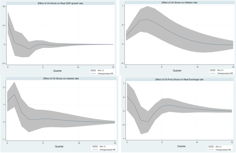Figure 6 presents the IRFs of each macroeconomic variable (in blue line) to a structural shock – an increase in global oil prices, with 95% CI (Shaded region).

Download: Download full-size image

Figure 6. IRFs of Each Variable’s Structural Shocks.

Real GDP growth exhibits a modest but statistically significant decline in response to an oil price shock. This negative effect is most pronounced within the first four quarters following the shock, with GDP gradually recovering toward baseline by around the 10th quarter. This finding reflects a short-run contractionary impact of oil price shocks on output, a result consistent with previous studies, which emphasize the muted but negative output effects of oil price shocks in advanced economies, especially when supported by stabilizing fiscal and monetary policies.

[6, 26]

Inflation displays a delayed yet persistent positive response, peaking around the third quarter post-shock. Although the confidence intervals widen over time, the response remains persistently above zero across several quarters, indicating a moderate but persistent inflationary effect. This result supports existing empirical literature that identifies lagged cost-push effects of oil prices on inflation such as Chen, 2009 and Alvarez et al., 2011 that document lagged inflationary responses to oil shocks in their results, under conditions of incomplete price adjustment and external cost transmission.

The real exchange rate reacts immediately and significantly, depreciating in the first two quarters after the shock. This reflects a terms-of-trade deterioration commonly experienced by oil-importing economies following price shocks. The exchange rate begins to stabilize after this point, with partial recovery seen by the 8th quarter. Similar trends are observed in studies which link oil shocks to currency depreciation and external imbalances.

[20]

The interest rate, representing monetary policy, rises sharply in the immediate aftermath of the oil shock, peaking within two quarters. This suggests that the Bank of England responds actively to contain the inflationary pressures generated by the external oil shock. Over time, it gradually returns toward its baseline level, consistent with an inflation-targeting central bank adjusting monetary policy as inflationary pressures subside.

[10]

Overall, the IRFs highlight a coherent and empirically consistent set of macroeconomic adjustments following an oil price shock. Output and competitiveness (via the exchange rate) respond immediately and negatively, while inflation and monetary policy exhibit slightly delayed but persistent responses.

5.3. Testing Robustness and Model Validity

To ensure the validity and robustness of the estimated SVAR model, several diagnostic tests were conducted, including checks for model stability, autocorrelation, and error normality. Table 9 summarizes the outcomes of these tests, while detailed outputs are provided in Appendix 3.

Table 9. Diagnostic Tests and Results.

Diagnostic	Test	Purpose	Statistic / Output	Result
Parameter Stability	Eigenvalue Test	Ensure model is dynamically stable	All eigenvalues < 1	Pass
Autocorrelation	Lagrange-Multiplier test	Check for serial correlation in residuals	Lag 1: p = 0.051	Pass
Autocorrelation	Lagrange-Multiplier test	Check for serial correlation in residuals	Lag 2: p = 0.080	Pass
Normality	Jarque–Bera Test	Assess whether residuals are normally distributed	χ² (10) = 4586.09, p = 0.000	Fail
	Skewness Test	Check for asymmetry in residuals	Significant skewness in most equations	Fail
	Kurtosis Test	Check for fat tails (leptokurtosis)	High kurtosis, e.g., GDP = 37.80	Fail
Overidentification	Likelihood-Ratio Test	Validate restrictions imposed in SVAR	Exactly identified (Just-identified model)	Not applicable (auto-pass)

The model satisfies the eigenvalue stability condition, with all roots lying inside the unit circle, confirming dynamic stability and validating the use of the VAR framework. The Lagrange-Multiplier test shows no significant autocorrelation, with p-values at lag 1 (0.051) and lag 2 (0.080), indicating that the chosen lag length of two is appropriate. Furthermore, as discussed earlier, the exact identification of the SVAR supports the identification strategy based on short-run restrictions. However, the model fails the normality tests. The Jarque-Bera test rejects the null hypothesis of normally distributed residuals at conventional significance levels (χ² = 4586.09, p < 0.01), supported by skewness and kurtosis tests. This is a known limitation, as non-normal residuals can undermine the reliability of CIs and hypothesis testing within the SVAR framework. Nonetheless, given the relatively large sample size (84 observations), the CLT provides robustness to asymptotic normality, allowing the estimators and IRFs to be interpreted with reasonable confidence.

Overall, the SVAR model demonstrates several strengths that support its use in analysing the macroeconomic impact of oil price shocks on UK’s economy. The model’s stability and lack of autocorrelation among the residuals reflects its well-specified temporal structure, ensuring that estimated responses to shocks are statistically sound over time. Additionally, the model’s exactly identifiable nature via Cholesky decomposition, grounded in NK theory, supports its interpretability of its estimates such as coefficients and IRFs. Furthermore, the model’s response function produced theoretically consistent and empirically backed results, capturing both immediate and lagged effects of structural shocks across key macroeconomic variables. These attributes make the model a credible tool for understanding the short-run impacts of oil prices on UK’s economy.

Nonetheless, some limitations remain. Most notably, it’s severed limitation of error non-normality, which may reduce the precision of standard inference—especially C.I.s derived under normality assumptions. While partially offset by CLT, this still introduces uncertainty in interpreting statistical significance. Additionally, the recursive identification strategy assumes a strict contemporaneous structure, which may not fully reflect real-world macroeconomic relationships. Lastly, the SVAR framework itself abstracts from underlying microeconomic foundations and assumes linear relationships, limiting its ability to capture non-linear or asymmetric effects of oil shocks, as noted in

[1]

. Despite these caveats, the model remains a useful and theoretically consistent framework for empirical analysis within the scope and level of this study.

6. Comparing Empirical Results to New Keynesian Predictions

We now compare the empirical results from the VAR-based analysis with the theoretical predictions derived from the NK model under the SOE framework. This comparison allows us to assess the consistency between observed and theoretical expectations, and to evaluate the explanatory power of the NK framework in the context of the UK economy.

To reiterate, the reduced form-VAR and IRF results reveal key macroeconomic patterns following a positive oil price shock. Real GDP contracts modestly but significantly in the short term. Inflation responds with a lag but shows a persistent increase. Meanwhile, interest rates tighten sharply in the short run before gradually stabilizing. The real exchange rate experiences an immediate and significant depreciation. Comparing to Table 2, these empirical findings align closely with the NK model's theoretical predictions, as summarized below:

1) Inflation: The empirical result of a lagged but sustained rise inflation aligns with NK expectations of cost-push inflation under nominal rigidities. Although the response is delayed, the direction and persistence are consistent with theoretical predictions and past empirical literature.

[3, 13]

2) Output (Real GDP): The observed short-run decline in output supports the NK view that oil shocks reduce aggregate demand through higher production costs and reduced real income, particularly in economies reliant on oil imports. This contraction is modest but statistically significant in the short run.

[26, 6]

3) Interest Rate: The sharp initial increase in the interest rate reflects a tightening monetary response to inflationary pressures, as anticipated under BoE’s inflation-targeting frameworks

[10]

. The gradual fall thereafter indicates that policymakers may weigh output stability alongside price stability, a trade-off in line with NK models with Taylor-type rules.

4) Exchange Rate: The immediate and significant depreciation of the exchange rate suggests that the terms-of-trade channel dominates, which is in line with the NK model's ambiguous prediction. For the UK—a net oil importer—the depreciation is expected and mirrors the external imbalances and inflation pass-through identified in open economy models.

[20]

Overall, the empirical results corroborate the main theoretical channels emphasized by the NK model. The direction and timing of the macroeconomic responses demonstrate the NK model’s continued relevance for analysing external price shocks in small open economies. While some deviations exist—such as the delayed inflation response—likely reflect structural features of the UK economy, global disinflationary trends, or post-crisis policy shifts. Thus, the evidence affirms the NK framework as a robust and relevant tool for analysing the short-run macroeconomic effects of external oil shocks on the UK economy.

7. Conclusion

This study set out to investigate the macroeconomic effects of oil price shocks on the UK economy during 2004–2024 within the theoretical framework of the NK model for SOE. Using a reduced form-VAR and SVAR methodology, we analysed the dynamic responses of real GDP, inflation, the interest rate, and the real exchange rate to exogenous oil price disturbances. Our findings broadly support the predictions of the NK model: oil shocks tend to generate short-run inflationary pressures, depress output, trigger monetary tightening, and cause real exchange rate depreciation, broadly consistent with standard theoretical expectations. Specifically, the empirical analysis revealed that oil price shocks exert a statistically significant contractionary effect on real GDP, a delayed but persistent upward effect on inflation, sharp monetary tightening and an immediate and significant depreciation of real exchange rate. Overall, these findings confirm the central role of oil price dynamics in influencing the short-run macroeconomic trajectory of the UK economy, validating key mechanisms of the NK model.

Despite the strengths of the analysis, the study has notable limitations. While the SVAR model satisfies stability and autocorrelation diagnostics, it fails to meet the normality assumption, introducing some uncertainty around standard inference. Moreover, the recursive identification strategy assumes strict contemporaneous causality, which may oversimplify real-world interactions. Additionally, the SVAR framework abstracts from non-linearities, financial frictions, and heterogeneous agent behaviour, all of which could influence the transmission of oil shocks but are not captured here.

From a policy perspective, the findings suggest that oil price shocks remain a significant source of macroeconomic volatility in the UK. Policymakers should remain vigilant in responding to oil-driven inflation pressures, particularly through adaptive monetary policy strategies that balance price stability with output stabilization. Moreover, given the sensitivity of the real exchange rate, maintaining external competitiveness through flexible exchange rate regimes and proactive fiscal measures becomes even more critical during periods of oil price volatility.

Finally, while this study offers valuable empirical evidence, it remains a bachelor-level academic work. Certain empirical limitations — including data restrictions, model simplifications, and methodological trade-offs — inevitably constrain the depth and generalizability of the findings. Future research could extend this work by incorporating non-linear models, financial sector frictions, or alternative identification schemes. Nevertheless, within its intended scope, this study provides a meaningful contribution to understanding the transmission of oil price shocks in the UK economy under a New Keynesian framework.

Abbreviations

ADF	Augmented Dickey-Fuller
AIC	Akaike Information Criteria
BoE	Bank of England
CAGR	Compounded Annual Growth Rate
CI	Confidence Interval
CLT	Central Limit Theorem
DSGE	Dynamic Stochastic General Equilibrium
FPE	Final Prediction Error
GFC	Global Financial Crisis
GDP	Gross Domestic Product
IRF	Impulse Response Function
LR	Likelihood-Ratio
MENA	Middle East and North Africa
NK	New Keynesian
NKIS	New Keynesian Investment Saving
NKPC	New Keynesian Phillips Curve
QoQ	Quarter on Quarter
RBC	Real Business Cycle
SBIC	Schwarz-Bayesian Information Criteria
SOE	Small Open Economy
SVAR	Structural Vector Auto-Regression
ToT	Terms of Trade
UK	United Kingdom
VAR	Vector Auto-Regression

Author Contributions

Vivek Singh Chauhan: Conceptualization, Data curation, Formal Analysis, Investigation, Methodology, Project administration, Resources, Software, Supervision, Validation, Visualization, Writing – original draft, Writing – review & editing

Conflicts of Interest

The authors declare no conflicts of interest.

Appendix

Appendix I: From Reduced Form-VAR Model to SVAR Model

In this appendix, we depict how we transformed or transition from reduced form-VAR to SVAR model. First, we take the reduced form-VAR equation, as below:

y_t=c+ ∑Φ_i y_(t-i) + ε_t

And assume, in accordance with enders (2004) {specifically chapter 5, subsection 10}, the following

ε_t= A^(-1) Bu_t

Or equivalently,

〖Aε〗_t= Bu_t

Where u_t represents the vector of structural shocks (calculated within SVAR), and ε_t are the reduced-form residuals obtained from the VAR. The matrices A and B are square matrices encoding the contemporaneous relationships among variables and the structure of the shocks, as discussed before.

[19]

We then multiply both sides of the reduced form-VAR equation with ‘A’, leading to the following:

Ay_t=Ac+ ∑〖AΦ〗_i y_(t-i) +〖Aε〗_t

Substituting 〖Aε〗_t for Bu_t and simplifying the model, we get the resulting equation, as below:

Ay_t= c ̃+ ∑Λ_i y_(t-i) + Bu_t

Where Λ_i=AΦ_i, representing the matrix of structural lagged coefficients and c ̃=Ac, representing transformed constant in SVAR.

Appendix II: Estimated Structural Coefficients by SVAR

Table of SVAR Estimated Coefficients.

Shock Source	Response Variable	Coefficient	Standard Error	p-value	95% Conf. Interval	Significance
Oil Price	Real Exchange Rate	-3.7161	1.7668	0.035	[-7.179, -0.253]	**
Oil Price	GDP	-0.0783	0.0201	0.000	[-0.118, -0.039]	***
Oil Price	Inflation	-1.2273	0.4532	0.007	[-2.115, -0.339]	***
Oil Price	Interest Rate	-0.7924	0.1864	0.000	[-1.158, -0.427]	***
Exchange Rate	GDP	-0.0008	0.0012	0.492	[-0.0033, 0.0016]
Exchange Rate	Inflation	0.0107	0.0255	0.675	[-0.0393, 0.0607]
Exchange Rate	Interest Rate	-0.0536	0.0101	0.000	[-0.0733, -0.0339]	***
GDP	Inflation	-3.0309	2.3031	0.188	[-7.545, 1.483]
GDP	Interest Rate	2.8994	0.9166	0.002	[1.103, 4.696]	***
Inflation	Interest Rate	-0.0407	0.0438	0.352	[-0.127, 0.045]
* 1%, 5%, * 10%, signifying p-value

Appendix III: Detailed Test Results

1) Parameter Stability (Eigenvalue test)

Table 11. Parameter Stability Results (Eigenvalue test).

Eigenvalue	Modulus
.7328765 +.1986767i	0.759329
.7328765 -.1986767i	0.759329
.5765869 +.2825686i	0.642104
.5765869 -.2825686i	0.642104
.2283412 +.5033808i	0.552749
.2283412 -.5033808i	0.552749
-.1807176 +.4717287i	0.50516
-.1807176 -.4717287i	0.50516
-.181604 +.06031088i	0.191357
-.181604 -.06031088i	0.191357

2) Autocorrelation (Lagrange-Multiplier test)

Table 12. Autocorrelation Results (Lagrange-Multiplier test).

Lag	chi2	Degrees of freedom	Prob > chi2
1	37.5221	25	0.05147
2	35.4554	25	0.08028
H0: No autocorrelation in lag order

3) Error Normality (Jarque-Bera test, skewness test and kurtosis test)

JB test –

Table 13. Jarque-Bera Test Results.

Equation	chi2	Degrees of freedom	Prob > chi2
D_lnOil	92.897	2	0.000
D_RealExchangerate	7.679	2	0.022
D_lnGDP	4400.068	2	0.000
Inflationrate	37.511	2	0.000
D_Interestrate	47.933	2	0.000
ALL	4586.088	10	0.000

Skewness test –

Table 14. Skewness Test Results.

Equation	Skewness	chi2	Degrees of freedom	Prob > chi2
D_lnOil	-1.466	29.029	1	0.000
D_RealExchangerate	-0.717	6.941	1	0.008
D_lnGDP	-4.808	312.113	1	0.000
Inflationrate	1.025	14.171	1	0.000
D_Interestrate	-0.724	7.076	1	0.008
ALL		369.331	5	0.000

Kurtosis test –

Table 15. Kurtosis Test Results

Equation	Kurtosis	chi2	Degrees of freedom	Prob > chi2
D_lnOil	7.350	63.868	1	0.000
D_RealExchangerate	3.468	0.738	1	0.390
D_lnGDP	37.803	4087.955	1	0.000
Inflationrate	5.630	23.340	1	0.000
D_Interestrate	6.479	40.857	1	0.000
ALL		4216.757	5	0.000

Appendix IV: STATA Commands

//Importing and preparing the DATA --------------

import excel "C:\Users\Unchi\OneDrive - University of Birmingham\Year 3\EEE\New EEE\DATA & STATA\DATASET\STATA data.xlsx", sheet("STATA Data") firstrow

gen tq = quarterly(Quarter, "YQ")

format tq%tq

tsset tq

//Testing the variables for stationary ----------

dfuller RealGDP

dfuller Inflationrate

dfuller Interestrate

dfuller RealExchangerate

dfuller OilPrice

//everything failed, not the appropriate test

//For test with lags

//Multiple varsoc for robustness in finding optimal lag

varsoc RealGDP

varsoc Inflationrate

varsoc Interestrate

varsoc RealExchangerate

varsoc OilPrice

varsoc RealGDP, maxlag(6)

varsoc Inflationrate, maxlag(6)

varsoc Interestrate, maxlag(6)

varsoc RealExchangerate, maxlag(6)

varsoc OilPrice, maxlag(6)

varsoc RealGDP, maxlag(8)

varsoc Inflationrate, maxlag(8)

varsoc Interestrate, maxlag(8)

varsoc RealExchangerate, maxlag(8)

varsoc OilPrice, maxlag(8)

dfuller RealGDP, lag(2)

dfuller Inflationrate, lag(2)

dfuller Interestrate, lag(2)

dfuller RealExchangerate, lag(2)

dfuller OilPrice, lag(2)

//Only Inflation rate (at 1%) and oil prices (at 10%) passed, however not the best appropriate test

//test with trends

dfuller RealGDP, trend

dfuller Inflationrate, trend

dfuller Interestrate, trend

dfuller RealExchangerate, trend

dfuller OilPrice, trend

//Only Real GDP passed, not the appropriate test

dfuller RealGDP, lag(2) trend

dfuller Inflationrate, lag(2) trend

dfuller Interestrate, lag(2) trend

dfuller RealExchangerate, lag(2) trend

dfuller OilPrice, lag(2) trend

//Only inlation rate passsed, near appropriate test

//transforming variables into rates and redoing the tests

gen lnGDP = ln(RealGDP)

gen lnOil = ln(OilPrice)

varsoc lnGDP, maxlag(6)

varsoc lnOil, maxlag(6)

varsoc lnGDP, maxlag(8)

varsoc lnOil, maxlag(8)

dfuller lnGDP, lag(2) trend

dfuller Inflationrate, lag(2) trend

dfuller Interestrate, lag(2) trend

dfuller RealExchangerate, lag(2) trend

dfuller lnOil, lag(2) trend

//Only inflation rate passed, near appropriate test

//Above test command is the most appropriate, with all variables in rates

gen D_lnGDP = D.lnGDP

gen D_Interestrate = D.Interestrate

gen D_RealExchangerate = D.RealExchangerate

gen D_lnOil = D.lnOil

//Doing the test on the diff. variables

varsoc D_lnGDP

varsoc D_Interestrate

varsoc D_RealExchangerate

varsoc D_lnOil

dfuller D_lnGDP, lag(1) trend

dfuller D_Interestrate, lag(1) trend

dfuller D_RealExchangerate, lag(1) trend

dfuller D_lnOil, trend

//All passed

//Summarizing the data --------------------------

asdoc sum lnGDP Inflationrate Interestrate RealExchangerate lnOil

//With every variable at I(1) except inflation rate (at I(0))

asdoc pwcorr lnGDP Inflationrate Interestrate RealExchangerate lnOil, sig

//Reduced form-VAR analysis ---------------------

varsoc D_lnGDP Inflationrate D_Interestrate D_RealExchangerate D_lnOil

varsoc D_lnGDP Inflationrate D_Interestrate D_RealExchangerate D_lnOil, maxlag(6)

varsoc D_lnGDP Inflationrate D_Interestrate D_RealExchangerate D_lnOil, maxlag(8)

asdoc var D_lnGDP Inflationrate D_Interestrate D_RealExchangerate D_lnOil

//Optimal lag is 1, already included in the command

//SVAR analysis with IRF ------------------------

//For already exsisting irf file -> erase [filename].irf

irf set newfile

//In case of already existing IRF file on system -> irf set SVARresult, replace

//Extreme case -> erase SVARresult.irf

//Making the restriction matrix, + cholesky recursive order.

matrix A = (1, 0, 0, 0, 0 \., 1, 0, 0, 0 \.,., 1, 0, 0 \.,.,., 1, 0 \.,.,.,., 1)

matrix B = (., 0, 0, 0, 0 \ 0,., 0, 0, 0 \ 0, 0,., 0, 0 \ 0, 0, 0,., 0 \ 0, 0, 0, 0,.)

asdoc svar D_lnOil D_RealExchangerate D_lnGDP Inflationrate D_Interestrate, aeq(A) beq(B)

//Model is exactly identifiable - All good!!

//Graphing IRF

irf create hehelol

irf describe

irf graph oirf, impulse(D_lnOil) response(D_RealExchangerate)

irf graph oirf, impulse(D_lnOil) response(D_lnGDP)

irf graph oirf, impulse(D_lnOil) response(Inflationrate)

irf graph oirf, impulse(D_lnOil) response(D_Interestrate)

//FECD to see the decomposition of the shock

irf graph fevd

//For detailed - > irf table fevd

//Stability

asdoc varstable

//All good!!

//Error non-normality

asdoc varnorm

//Heavy error non-normality - Not good...

//Autocorrelation

asdoc varlmar

//Close call on lag 1 - All good!!

References

[1]	Abubakar, A. B., Karimu, S. and Mamman, S. O. (2024) ‘Inflation effects of oil and gas prices in the UK: Symmetries and asymmetries’, Utilities Policy, 90, pp. 101803–101803. Available at: https://doi.org/10.1016/j.jup.2024.101803
[2]	Ahmed, R. et al. (2023) ‘Inflation, oil prices, and economic activity in recent crisis: Evidence from the UK’, Energy Economics, 126(1), p. 106918. Available at: https://doi.org/10.1016/j.eneco.2023.106918
[3]	Alvarez, F., Le Bihan, H. and Lippi, F. (2016) ‘The Real Effects of Monetary Shocks in Sticky Price Models: A Sufficient Statistic Approach’, American Economic Review, 106(10), pp. 2817–2851. Available at: https://doi.org/10.1257/aer.20140500
[4]	Annut, A. and Campbell, A. (2024) Chapter 3: Oil and Oil Products. Available at: https://assets.publishing.service.gov.uk/media/66a7a451ce1fd0da7b592eb8/DUKES_2024_Chapter_3.pdf
[5]	Ball, L. and Gregory, M. N. (2025) ‘Asymmetric Price Adjustment and Economic Fluctuations’, Economic Journal, 104(423), pp. 247–61. Available at: https://econpapers.repec.org/article/ecjeconjl/v_3a104_3ay_3a1994_3ai_3a423_3ap_3a247-61.htm (Accessed: 5 April 2025).
[6]	Baumeister, C. and Peersman, G. (2013) ‘Time-Varying Effects of Oil Supply Shocks on the US Economy’, American Economic Journal: Macroeconomics, 5(4), pp. 1–28. Available at: https://www.jstor.org/stable/43189560
[7]	Bernanke, B. S., Gertler, M. and Watson, M. (1997) ‘Systematic Monetary Policy and the Effects of Oil Price Shocks’, Brookings Papers on Economic Activity, 1997(1), p. 91. Available at: https://doi.org/10.2307/2534702
[8]	Berument, H., Ceylan, N. and Dogan, N. (2025) ‘The Impact of Oil Price Shocks on the Economic Growth of Selected MENA1 Countries’, The Energy Journal, Volume 31(Number 1), pp. 149–176. Available at: https://econpapers.repec.org/article/aenjournl/2010v31-01-a07.htm (Accessed: 5 April 2025).
[9]	Bolton, P. (2022) ‘Oil Prices’, commonslibrary.parliament.uk [Preprint]. Available at: https://commonslibrary.parliament.uk/research-briefings/sn02106/
[10]	Burr, N. and Willems, T. (2024) About a rate of (general) interest: how monetary policy transmits. Available at: https://www.bankofengland.co.uk/quarterly-bulletin/2024/2024/about-a-rate-of-general-interest-how-monetary-policy-transmits (Accessed: 25 April 2025).
[11]	Campa, J. M. and Goldberg, L. S. (2005) ‘Exchange Rate Pass-through into Import Prices’, The Review of Economics and Statistics, 87(4), pp. 679–690. Available at: https://www.jstor.org/stable/40042885
[12]	Cashin, P. et al. (2025) ‘The differential effects of oil demand and supply shocks on the global economy’, Energy Economics, 44(C), pp. 113–134. Available at: https://econpapers.repec.org/article/eeeeneeco/v_3a44_3ay_3a2014_3ai_3ac_3ap_3a113-134.htm (Accessed: 5 April 2025).
[13]	Chen, S.-S. (2025) ‘Oil price pass-through into inflation’, Energy Economics, 31(1), pp. 126–133. Available at: https://econpapers.repec.org/article/eeeeneeco/v_3a31_3ay_3a2009_3ai_3a1_3ap_3a126-133.htm (Accessed: 25 April 2025).
[14]	Christiano, L. J., Motto, R. and Rostagno, M. (2014) ‘Risk Shocks’, The American Economic Review, 104(1), pp. 27–65. Available at: https://doi.org/10.2307/42920687
[15]	Christiano, Lawrence J., Eichenbaum, M. and Evans, Charles L. (2005) ‘Nominal Rigidities and the Dynamic Effects of a Shock to Monetary Policy’, Journal of Political Economy, 113(1), pp. 1–45. Available at: https://doi.org/10.1086/426038
[16]	Clark, D. (2025) Inflation rate for the Consumer Price Index (CPI) in the United Kingdom from January 2000 to January 2025, Statista. Available at: https://www.statista.com/statistics/306648/inflation-rate-consumer-price-index-cpi-united-kingdom-uk/
[17]	Coibion, O. and Gorodnichenko, Y. (2015) ‘Information Rigidity and the Expectations Formation Process: A Simple Framework and New Facts’, The American Economic Review, 105(8), pp. 2644–2678. Available at: https://doi.org/10.2307/43821351
[18]	Corsetti, G., Dedola, L. and Leduc, S. (2025) ‘International Risk Sharing and the Transmission of Productivity Shocks’, The Review of Economic Studies, 75(2), pp. 443–473. Available at: https://econpapers.repec.org/article/ouprestud/v_3a75_3ay_3a2008_3ai_3a2_3ap_3a443-473.htm (Accessed: 5 April 2025).
[19]	Enders, W. (2014) Applied econometric time series. 4th edn. Hoboken: Wiley, Cop.
[20]	Erceg, M. (2011) ‘Oil shocks and external adjustment’, Journal of International Economics, 83(2), pp. 168–184. Available at: https://ideas.repec.org/a/eee/inecon/v83y2011i2p168-184.html (Accessed: 25 April 2025).
[21]	Fuhrer, J. C. (2010) ‘Inflation Persistence’, Handbook of Monetary Economics, 3, pp. 423–486. Available at: https://doi.org/10.1016/b978-0-444-53238-1.00009-0
[22]	Galí, J. (2015) Monetary policy, inflation, and the business cycle: an introduction to the new Keynesian framework and its applications. Princeton; Oxford: Princeton University Press. Available at: https://perhuaman.files.wordpress.com/2014/06/gali_polc3adtica_monetaria.pdf
[23]	Galí, J. and Gertler, M. (2000) NBER WORKING PAPER SERIES INFLATION DYNAMICS: A STRUCTURAL ECONOMETRIC ANALYSIS. Available at: https://www.nber.org/system/files/working_papers/w7551/w7551.pdf
[24]	International Monetary Fund (1955) Real Gross Domestic Product for Great Britain, FRED, Federal Reserve Bank of St. Louis. Available at: https://fred.stlouisfed.org/series/NGDPRSAXDCGBQ (Accessed: 6 April 2025).
[25]	International Monetary Fund (1980) Global price of Brent Crude, FRED, Federal Reserve Bank of St. Louis. Available at: https://fred.stlouisfed.org/series/POILBREUSDQ (Accessed: 6 April 2025).
[26]	Kilian, L. (2008) ‘The Economic Effects of Energy Price Shocks’, Journal of Economic Literature, 46(4), pp. 871–909. Available at: https://doi.org/10.1257/jel.46.4.871
[27]	Killian, L. and Vega, C. (2024) DO ENERGY PRICES RESPOND TO U.S. MACROECONOMIC NEWS? A TEST OF THE HYPOTHESIS OF PREDETERMINED ENERGY PRICES on JSTOR, Jstor.org. Available at: https://www.jstor.org/stable/23015961
[28]	Lorusso, M. and Pieroni, L. (2018) ‘Causes and consequences of oil price shocks on the UK economy’, Economic Modelling, 72, pp. 223–236. Available at: https://doi.org/10.1016/j.econmod.2018.01.018
[29]	Lubik, T. A. and Schorfheide, F. (2007) ‘Do central banks respond to exchange rate movements? A structural investigation’, Journal of Monetary Economics, 54(4), pp. 1069–1087. Available at: https://doi.org/10.1016/j.jmoneco.2006.01.009
[30]	Lutz Kilian and Helmut Lütkepohl (2017) Structural Vector Autoregressive Analysis. Cambridge University Press.
[31]	Millard, S. and Shakir, T. (2013) ‘Oil Shocks and the UK Economy: The Changing Nature of Shocks and Impact Over Time’, SSRN Electronic Journal [Preprint]. Available at: https://doi.org/10.2139/ssrn.2313021
[32]	Obstfeld, M. and Rogoff, K. (2000) ‘Title: The Six Major Puzzles in International Macroeconomics: Is There a Common Cause? The Si x Major Puzzles i n International Macroeconomics: I s There a Common Cause?’, 15, pp. 0–262. Available at: https://www.nber.org/system/files/chapters/c11059/c11059.pdf
[33]	Preston, A. (2010) ‘Can structural small open-economy models account for the influence of foreign disturbances?’, Journal of International Economics, 81(1), pp. 61–74. Available at: https://ideas.repec.org/a/eee/inecon/v81y2010i1p61-74.html (Accessed: 5 April 2025).
[34]	Romer, C. D. and Romer, D. H. (2004) ‘A New Measure of Monetary Shocks: Derivation and Implications’, American Economic Review, 94(4), pp. 1055–1084. Available at: https://doi.org/10.1257/0002828042002651
[35]	Smets, F. and Wouters, R. (2007) ‘Shocks and Frictions in US Business Cycles: A Bayesian DSGE Approach’, American Economic Review, 97(3), pp. 586–606. Available at: https://doi.org/10.1257/aer.97.3.586
[36]	Statista Research Department (2024a) Countries with the highest oil consumption 2019, Statista. Available at: https://www.statista.com/statistics/271622/countries-with-the-highest-oil-consumption-in-2012/ (Accessed: 6 April 2025).
[37]	Statista Research Department (2024b) UK: oil consumption 2021, Statista. Available at: https://www.statista.com/statistics/264411/oil-consumption-in-the-united-kingdom/ (Accessed: 6 April 2025).
[38]	UK became a net importer of petroleum products in 2013 - Today in Energy - U.S. Energy Information Administration (EIA) (2014) www.eia.gov. Available at: https://www.eia.gov/todayinenergy/detail.php?id=16971

Cite This Article

Plain Text BibTeX RIS

APA Style

Chauhan, V. S. (2026). The UK Economy and Oil Price Shocks: An Empirical Assessment Under the New Keynesian Framework. International Journal of Economy, Energy and Environment, 11(3), 74-96. https://doi.org/10.11648/j.ijeee.20261103.13

Copy | Download

ACS Style

Chauhan, V. S. The UK Economy and Oil Price Shocks: An Empirical Assessment Under the New Keynesian Framework. Int. J. Econ. Energy Environ. 2026, 11(3), 74-96. doi: 10.11648/j.ijeee.20261103.13

Copy | Download

AMA Style

Chauhan VS. The UK Economy and Oil Price Shocks: An Empirical Assessment Under the New Keynesian Framework. Int J Econ Energy Environ. 2026;11(3):74-96. doi: 10.11648/j.ijeee.20261103.13

Copy | Download

@article{10.11648/j.ijeee.20261103.13,
  author = {Vivek Singh Chauhan},
  title = {The UK Economy and Oil Price Shocks: An Empirical Assessment Under the New Keynesian Framework},
  journal = {International Journal of Economy, Energy and Environment},
  volume = {11},
  number = {3},
  pages = {74-96},
  doi = {10.11648/j.ijeee.20261103.13},
  url = {https://doi.org/10.11648/j.ijeee.20261103.13},
  eprint = {https://article.sciencepublishinggroup.com/pdf/10.11648.j.ijeee.20261103.13},
  abstract = {This study investigates the macroeconomic effects of the global oil price shocks on the United Kingdom from 2004 to 2024 within the framework of the New Keynesian (NK) model for small open economies. Employing reduced-form VAR and SVAR approaches, we analyse the dynamic responses of real GDP, inflation, the interest rate, and the real exchange rate to exogenous oil price movements. Beyond interpreting these effects, the study critically assesses how closely real-world outcomes align with NK model predictions. From VAR analysis, our findings (by interpretating impulse-response functions) largely validate the NK framework. For a positive oil price shock, it results in cost-push inflation by raising firms' marginal production costs. Inflation increases persistently in the short to medium term, while output contracts due to declining real income and tighter financial conditions. Monetary policy responds endogenously through interest rate hikes aimed at stabilizing inflation expectations, amplifying short-run output losses. The real exchange rate depreciates following adverse oil shocks, reflecting both deteriorating trade conditions and monetary tightening dynamics. While findings largely validate the NK model's qualitative implications, the study has its own diagnostic limitations such as non-normal residuals and model simplification. Overall, the study provides contribution to empirical evidence validating the relevance of the NK model framework, particularly for understanding oil price shocks to an open small economy.},
 year = {2026}
}

Copy | Download

TY  - JOUR
T1  - The UK Economy and Oil Price Shocks: An Empirical Assessment Under the New Keynesian Framework
AU  - Vivek Singh Chauhan
Y1  - 2026/06/18
PY  - 2026
N1  - https://doi.org/10.11648/j.ijeee.20261103.13
DO  - 10.11648/j.ijeee.20261103.13
T2  - International Journal of Economy, Energy and Environment
JF  - International Journal of Economy, Energy and Environment
JO  - International Journal of Economy, Energy and Environment
SP  - 74
EP  - 96
PB  - Science Publishing Group
SN  - 2575-5021
UR  - https://doi.org/10.11648/j.ijeee.20261103.13
AB  - This study investigates the macroeconomic effects of the global oil price shocks on the United Kingdom from 2004 to 2024 within the framework of the New Keynesian (NK) model for small open economies. Employing reduced-form VAR and SVAR approaches, we analyse the dynamic responses of real GDP, inflation, the interest rate, and the real exchange rate to exogenous oil price movements. Beyond interpreting these effects, the study critically assesses how closely real-world outcomes align with NK model predictions. From VAR analysis, our findings (by interpretating impulse-response functions) largely validate the NK framework. For a positive oil price shock, it results in cost-push inflation by raising firms' marginal production costs. Inflation increases persistently in the short to medium term, while output contracts due to declining real income and tighter financial conditions. Monetary policy responds endogenously through interest rate hikes aimed at stabilizing inflation expectations, amplifying short-run output losses. The real exchange rate depreciates following adverse oil shocks, reflecting both deteriorating trade conditions and monetary tightening dynamics. While findings largely validate the NK model's qualitative implications, the study has its own diagnostic limitations such as non-normal residuals and model simplification. Overall, the study provides contribution to empirical evidence validating the relevance of the NK model framework, particularly for understanding oil price shocks to an open small economy.
VL  - 11
IS  - 3
ER  -

Copy | Download

Author Information

Vivek Singh Chauhan

University of Birmingham, Dubai, UAE

Contact Email

http://orcid.org/0009-0009-0647-370X

Download PDF

Submit an Article

Plain Text BibTeX RIS

APA Style

Chauhan, V. S. (2026). The UK Economy and Oil Price Shocks: An Empirical Assessment Under the New Keynesian Framework. International Journal of Economy, Energy and Environment, 11(3), 74-96. https://doi.org/10.11648/j.ijeee.20261103.13

Copy | Download

ACS Style

Chauhan, V. S. The UK Economy and Oil Price Shocks: An Empirical Assessment Under the New Keynesian Framework. Int. J. Econ. Energy Environ. 2026, 11(3), 74-96. doi: 10.11648/j.ijeee.20261103.13

Copy | Download

AMA Style

Chauhan VS. The UK Economy and Oil Price Shocks: An Empirical Assessment Under the New Keynesian Framework. Int J Econ Energy Environ. 2026;11(3):74-96. doi: 10.11648/j.ijeee.20261103.13

Copy | Download

@article{10.11648/j.ijeee.20261103.13,
  author = {Vivek Singh Chauhan},
  title = {The UK Economy and Oil Price Shocks: An Empirical Assessment Under the New Keynesian Framework},
  journal = {International Journal of Economy, Energy and Environment},
  volume = {11},
  number = {3},
  pages = {74-96},
  doi = {10.11648/j.ijeee.20261103.13},
  url = {https://doi.org/10.11648/j.ijeee.20261103.13},
  eprint = {https://article.sciencepublishinggroup.com/pdf/10.11648.j.ijeee.20261103.13},
  abstract = {This study investigates the macroeconomic effects of the global oil price shocks on the United Kingdom from 2004 to 2024 within the framework of the New Keynesian (NK) model for small open economies. Employing reduced-form VAR and SVAR approaches, we analyse the dynamic responses of real GDP, inflation, the interest rate, and the real exchange rate to exogenous oil price movements. Beyond interpreting these effects, the study critically assesses how closely real-world outcomes align with NK model predictions. From VAR analysis, our findings (by interpretating impulse-response functions) largely validate the NK framework. For a positive oil price shock, it results in cost-push inflation by raising firms' marginal production costs. Inflation increases persistently in the short to medium term, while output contracts due to declining real income and tighter financial conditions. Monetary policy responds endogenously through interest rate hikes aimed at stabilizing inflation expectations, amplifying short-run output losses. The real exchange rate depreciates following adverse oil shocks, reflecting both deteriorating trade conditions and monetary tightening dynamics. While findings largely validate the NK model's qualitative implications, the study has its own diagnostic limitations such as non-normal residuals and model simplification. Overall, the study provides contribution to empirical evidence validating the relevance of the NK model framework, particularly for understanding oil price shocks to an open small economy.},
 year = {2026}
}

Copy | Download

TY  - JOUR
T1  - The UK Economy and Oil Price Shocks: An Empirical Assessment Under the New Keynesian Framework
AU  - Vivek Singh Chauhan
Y1  - 2026/06/18
PY  - 2026
N1  - https://doi.org/10.11648/j.ijeee.20261103.13
DO  - 10.11648/j.ijeee.20261103.13
T2  - International Journal of Economy, Energy and Environment
JF  - International Journal of Economy, Energy and Environment
JO  - International Journal of Economy, Energy and Environment
SP  - 74
EP  - 96
PB  - Science Publishing Group
SN  - 2575-5021
UR  - https://doi.org/10.11648/j.ijeee.20261103.13
AB  - This study investigates the macroeconomic effects of the global oil price shocks on the United Kingdom from 2004 to 2024 within the framework of the New Keynesian (NK) model for small open economies. Employing reduced-form VAR and SVAR approaches, we analyse the dynamic responses of real GDP, inflation, the interest rate, and the real exchange rate to exogenous oil price movements. Beyond interpreting these effects, the study critically assesses how closely real-world outcomes align with NK model predictions. From VAR analysis, our findings (by interpretating impulse-response functions) largely validate the NK framework. For a positive oil price shock, it results in cost-push inflation by raising firms' marginal production costs. Inflation increases persistently in the short to medium term, while output contracts due to declining real income and tighter financial conditions. Monetary policy responds endogenously through interest rate hikes aimed at stabilizing inflation expectations, amplifying short-run output losses. The real exchange rate depreciates following adverse oil shocks, reflecting both deteriorating trade conditions and monetary tightening dynamics. While findings largely validate the NK model's qualitative implications, the study has its own diagnostic limitations such as non-normal residuals and model simplification. Overall, the study provides contribution to empirical evidence validating the relevance of the NK model framework, particularly for understanding oil price shocks to an open small economy.
VL  - 11
IS  - 3
ER  -

Copy | Download