2. Literature Review
In the past ten years, the link between renewable energy use and economic growth has attracted increasing attention in the fields of economics, especially in light of global shifts towards more sustainable development models. Most of these studies have focused on the impact of energy consumption on GDP or the causal relationship between the two variables. However, little research has been done on the association between renewable energy use and inclusive growth, highlighting the importance of further research on this topic, especially in developing contexts such as African countries or the Egyptian economy
| [5] | Ibrahiem, D. M. (2015). Renewable electricity consumption, foreign direct investment and economic growth in Egypt: An ARDL approach. Procedia Economics and Finance, 30, 313-323. |
| [6] | Wesseh Jr, P. K., & Lin, B. (2018). Energy consumption, fuel substitution, technical change, and economic growth: Implications for CO2 mitigation in Egypt. Energy Policy, 117, 340-347. |
[5, 6]
.
The literature on energy-economic growth nexus tests the following four basic hypotheses: (a) growth hypothesis, (b) feedback hypothesis, (c) neutrality hypothesis and (d) conservation hypothesis. The growth hypothesis prevails in the event there is one-directional causation from economic growth to energy consumption. In compliance with the hypothesis, curbing energy consumption brakes economic growth, while encouraging energy consumption promotes economic growth. The feedback hypothesis is interested in a two-way causality between economic growth and energy consumption. In this case, energy consumption and economic growth are jointly determined and affected at the same point in time. According to the neutrality hypothesis, there is no causality between the two variables that suggests economic growth is independent of energy policies. The conservation hypothesis speculates a one-way causality from economic growth to energy consumption. The conservation hypothesis expects that policy aimed at energy conservation will not adversely affect economic growth.
| [7] | Kouton, J. (2021). Renewable energy consumption and inclusive growth in Sub-Saharan Africa: Evidence from a system GMM approach. Renewable Energy, 179, 678-691. |
[7]
We explain below some tests of these alternative hypotheses conducted in this section of the article.
Apergis, N., & Payne, J. E.
| [8] | Apergis, N., & Payne, J. E. (2010). Renewable energy consumption and economic growth: Evidence from a panel of OECD countries. Energy Policy, 38(1), 656-660. |
[8]
used panel data analysis to test the relationship between economic growth and renewable energy consumption in thirteen Eurasian countries from 1992 to 2007. The results showed bi-directional causality between the two variables in both the short and long run, suggesting that not only does renewable energy stimulate growth, but growth itself promotes the expansion of clean energy use. In a subsequent study, Apergis, N., & Payne, J. E.
| [9] | Apergis, N., & Payne, J. E. (2011). The renewable energy consumption-growth nexus in Central America. Applied Energy, 88(1), 343-347. |
[9]
identified a long-term relationship between renewable energy consumption and economic growth in 25 developed and 55 developing economies over the period 1990-2007. They used cointegration tests and determined that a 1% increase in renewable energy consumption leads to a 0.265% increase in GDP in developed countries and 0.429% in developing countries. The results also indicated a bidirectional causality in developed countries, while this relationship was not observed in developing countries, due to low levels of renewable energy utilization. Shahbaz, M. et al.
| [10] | Shahbaz, M., Loganathan, N., Zeshan, M., & Zaman, K. (2015). Does renewable energy consumption add in economic growth? An application of auto-regressive distributed lag model in Pakistan. Renewable and Sustainable Energy Reviews, 44, 576-585. |
[10]
confirmed the long-term relationship between economic growth and renewable energy consumption in the case of Pakistan, where they used an autoregressive distributed lag (ARDL) model on data spanning from 1972 to 2011. The results showed a bi-directional causality, but the impact of renewable energy on economic growth was more significant than the reverse, highlighting the importance of investing in renewable energy as a driving force for growth in developing countries.
By analyzing data for 34 OECD countries during the period 1990-2010, Inglesi-Lotz, R.
| [11] | Inglesi-Lotz, R. (2016). The impact of renewable energy consumption to economic growth: A panel data application. Energy Economics, 53, 58-63. |
[11]
found that the level of renewable energy consumption and its share in the total energy mix has clear positive effects on economic growth. The study recommended that policies that support the integration of renewable energy into the economic structure would promote aggregate and sustainable growth in the long term. In the Nigerian context, Maji, I. K.
| [12] | Maji, I. K. (2015). Does clean energy contribute to economic growth? Evidence from Nigeria. Energy Reports, 1, 145-150. |
[12]
conducted an analytical study on the relationship between multiple types of energy sources and economic growth over the period 1971-2011, and concluded that clean energy sources such as nuclear and alternative energy had a negative impact on economic growth, while combustible renewable energy (such as biomass) showed a positive and significant impact. The study pointed to the need for effective infrastructure to integrate clean energy into the national production model. Using advanced modeling techniques FMOLS and DOLS, Bhattacharya, M. et al.
| [13] | Bhattacharya, M., Paramati, S. R., Ozturk, I., & Bhattacharya, S. (2016). The effect of renewable energy consumption on economic growth: Evidence from top 38 countries. Applied Energy, 162, 733-741. |
[13]
showed that the relationship between renewable energy consumption and economic growth varies from country to country across a sample of 38 countries. In some cases, the relationship was positive as a result of job creation through renewable energy, while in other cases the effect was negative due to the low level of renewable energy use in the national energy mix, emphasizing the importance of the institutional environment in the success of sustainable energy policies. Ozcan, B., & Ozturk, I.
| [14] | Ozcan, B., & Ozturk, I. (2019). Renewable energy consumption-economic growth nexus in emerging countries: A bootstrap panel causality test. Renewable and Sustainable Energy Reviews, 104, 30-37. |
[14]
examined the relationship between economic growth and renewable energy consumption in 17 emerging economies during the period from 1990 to 2016 through the Bootstrap Panel Causality Test. The evidence supported the neutrality hypothesis in 16 countries, i.e., no causality between the two variables, while only Poland revealed a one-way relationship from renewable energy consumption to economic development, suggesting that renewable energy consumption continues to be of limited importance in most of these countries in view of incomplete institutional and economic integration.
Maji, I. K. et al. (2019)
| [15] | Maji, I. K., Sulaiman, C., & Abdul-Rahim, A. S. (2019). Renewable energy consumption and economic growth nexus: A fresh evidence from West Africa. Energy Reports, 5, 384-392. |
[15]
examined 15 West African countries from 1995-2014 using a dynamic ordinary least squares (DOLS) regression model. Results showed that consumption of renewable energy negatively affects economic growth as countries utilize traditional primary energy sources such as wood and charcoal, whose negative effect is on productive efficiency and limits potential development. The scientists proposed the need to construct energy infrastructure and grow reliance on new and more efficient types of renewable energy. Omri, A. et al. (2015)
| [16] | Omri, A., Daly, S., Rault, C., & Chaibi, A. (2015). Financial development, environmental quality, trade and economic growth: What causes what in MENA countries. Energy Economics, 48, 242-252. |
[16]
used a dynamic GMM model to analyze the causal relationship between renewable energy and economic growth in 17 developed and developing countries during the period 1990-2011. The study showed that the relationships are heterogeneous: Countries such as Hungary, India, and Japan experienced a causal relationship from energy to growth, while in other countries such as Argentina and Switzerland, growth was the driver of renewable energy consumption. Bi-directional relationships emerged in countries such as the US and Canada, while no causal relationships emerged in Finland and Brazil. These results reflect the different regulatory frameworks and energy policies between countries.
Aydin, M.
| [17] | Aydin, M. (2019). Renewable and non-renewable electricity consumption-economic growth nexus: Evidence from OECD countries. Renewable Energy, 136, 599-606. |
[17]
conducted an in-depth analysis of the relationship between electricity consumption from renewable sources and economic growth in 26 OECD countries during the period 1980-2015, using frequency causality and Dumitrescu-Hurlin tests. The study showed a bi-directional causality, confirming the feedback hypothesis and highlighting the importance of renewable electricity consumption as a stable source of growth in developed economies. Vural, G.
| [18] | Vural, G. (2020). The effects of renewable energy consumption on economic growth in Sub-Saharan African countries. Environmental Science and Pollution Research, 27(28), 35396-35406. |
[18]
targeted six countries, namely Nigeria, South Africa, Sudan, Kenya, Gabon, and Madagascar during the period 1990-2015. The study used advanced integration techniques such as Pedroni and FMOLS and found a strong positive relationship between renewable energy consumption and economic growth, indicating that the orderly exploitation of renewable potential in these countries could be a critical driver for improving economic performance and expanding employment prospects. Kahia, M. et al. (2017)
| [19] | Kahia, M., Aïssa, M. S. B., & Lanouar, C. (2017). Renewable and non-renewable energy use-economic growth nexus: The case of MENA Net Oil Importing Countries. Renewable and Sustainable Energy Reviews, 71, 127-140. |
[19]
studied the relationship between renewable energy and growth in 11 MENA countries dependent on oil imports during the period 1980-2012. Using error correction models and Granger causality tests, the study found bi-directional causality, suggesting that renewable energy expansion can reduce dependence on imported oil and support sustainable economic growth in these countries.
As part of the studies that examined temporal causality, Saidi, K., & Mbarek, M. B.
| [20] | Saidi, K., & Mbarek, M. B. (2016). Nuclear energy, renewable energy, CO2 emissions, and economic growth for nine developed countries: Evidence from panel Granger causality tests. Progress in Nuclear Energy, 88, 364-374. |
[20]
examined nine developed countries during the period 1990-2013 using dynamic panel models. They found a unidirectional causality from renewable energy consumption to GDP per capita in the short run, while a bidirectional causality was observed in the long run, reflecting the cumulative effect of clean energy consumption in supporting growth over the extended time horizon. Bhat, J. A.
| [21] | Bhat, J. A. (2018). Renewable and non-renewable energy consumption-impact on economic growth in five emerging market economies. Environmental Economics and Policy Studies, 20(3), 705-736. |
[21]
focused on five major emerging economies (Brazil, Russia, India, China, India, China, and South Africa) during the period 1992-2016, using pooled regression models and cointegration tests. His results showed a statistically insignificant positive relationship between renewable energy consumption and economic growth. The researcher explained this by the weak investments in renewable energy or its limited impact within the overall productive structure in those countries. Rasoulinezhad, E., & Saboori, B.
| [22] | Rasoulinezhad, E., & Saboori, B. (2018). Panel estimation for renewable energy consumption, economic growth, CO2 emissions, the composite trade intensity, and financial openness of the Commonwealth of Independent States. Environmental Science and Pollution Research, 25(18), 17354-17370. |
[22]
analyzed the relationship between renewable energy consumption and economic growth in 13 CIS countries during 1992-2015 using FMOLS and DOLS models. The results confirmed a long-term unidirectional relationship from renewable energy to growth, which supports the growth hypothesis and indicates the importance of including renewable energy in the economic development plans of those countries emerging from the era of centralized economies.
In a study more focused on the Arab region, Charfeddine, L., & Kahia, M.
| [23] | Charfeddine, L., & Kahia, M. (2019). Impact of renewable energy consumption and financial development on CO2 emissions and economic growth in the MENA region: A panel vector autoregressive (PVAR) analysis. Renewable Energy, 139, 198-213. |
[23]
, analyzing data for 24 MENA countries during the period 1980-2015, found that the positive impact of renewable energy consumption on economic growth was weak. They used VAR models and attributed this weakness to the absence of effective infrastructure or supportive legislation, highlighting the importance of creating a favorable regulatory and investment environment for clean energy in the region. Rahman, M. M., & Velayutham, E.
| [24] | Rahman, M. M., & Velayutham, E. (2020). Renewable and non-renewable energy consumption-economic growth nexus: New evidence from South Asia. Energy Reports, 6, 424-432. |
[24]
tested the relationship in five South Asian countries (India, Pakistan, Bangladesh, Nepal, and Sri Lanka) during the period 1990-2014 using FMOLS and DOLS models and causality tests. The results showed a clear positive effect of renewable energy consumption on growth, with a unidirectional causality from growth to energy, confirming that economic improvement may lead to increased demand for clean energy.
Although much work has been done that has examined the impact of renewable energy consumption on GDP or the causal relationships between energy and growth, studies that have examined the relationship between renewable energy consumption and inclusive growth are still relatively few. One of the few studies that have addressed this issue is Kouton, J.
| [7] | Kouton, J. (2021). Renewable energy consumption and inclusive growth in Sub-Saharan Africa: Evidence from a system GMM approach. Renewable Energy, 179, 678-691. |
[7]
, which investigated the impact of renewable energy use on inclusive growth in 44 African countries from 1991 to 2015. The study relied on estimating a dynamic panel model using the Generalized Method of Moments (System GMM), and the real value of GDP per worker was used as a proxy for inclusive growth, reflecting both productivity and employment. The results revealed a strong positive relationship between renewable energy consumption and inclusive growth, especially in countries with low levels of economic inclusion. The study confirmed that the expansion of renewable energy not only affects macroeconomic growth, but also improves income distribution, promotes social justice, and stimulates job creation, especially in rural and marginalized areas. It also shows that increased investment in renewable energy leads to higher productive efficiency and higher returns to labor, both directly through employment and indirectly through improved infrastructure and services. The study also highlighted the importance of the interaction between renewable energy and institutional components, such as economic stability and governance, as a mediator that enhances the ability of renewable energy to spur inclusive growth. It concludes that African countries' shift towards clean energy can be a strategic entry point for reducing the development gap and achieving the SDGs.
Cui et al.
| [25] | Cui, L., Weng, S., & Song, M. (2022). Financial inclusion, renewable energy consumption, and inclusive growth: Cross-country evidence. Energy Efficiency, 15(6), 43. |
[25]
examined the relationship between renewable energy consumption and inclusive growth by analysing panel balance data for a sample of 40 countries (22 developed and 18 developing countries) during the period 2010 to 2020. The researchers used the Spatial Durbin Model (SDM) to analyse the relationship, taking into account spatial effects and economic spillovers between neighbouring countries. The results revealed that renewable energy consumption contributes positively to inclusive growth. Renewable energy consumption contributes to optimising the energy structure, which promotes sustainable and more equitably distributed economic growth.
Ghose et al.
| [2] | Ghouse, G., Aslam, A., & Bhatti, M. I. (2022). Green energy consumption and inclusive growth: A comprehensive analysis of multi-country study. Frontiers in Energy Research, 10, 939920. |
[2]
investigated the relationship between green energy consumption and inclusive growth by analysing panel balance data for 83 countries classified by the World Bank as high-, middle-, and low-income countries during the period 2010-2020. The researchers used a dynamic panel data model using the Generalised Method of Modelling (GMM) to address the issue of endogeneity, while constructing composite indicators for social inclusion, digital inclusion, quality of institutions, and inclusive growth. The results revealed that green energy consumption contributes positively and significantly to inclusive growth, but the effect was stronger in high-income countries compared to middle- and low-income countries. The study also showed that the interaction between social inclusion and green energy, as well as between digital inclusion and green energy, has a significant positive impact on inclusive growth across all income groups, suggesting that raising social and digital awareness supports the shift towards clean energy and enhances inclusive growth outcomes. In addition, the quality of institutions, trade openness, investment, and education were all found to be supportive of inclusive growth, while inflation has a significant negative effect only in low-income countries. The researchers emphasised that institutional weaknesses in poor countries limit the impact of green energy on achieving inclusive and sustainable growth. The study recommended that developing countries should adopt policies to improve social and digital inclusion, enhance the quality of institutions, and invest heavily in renewable energy in order to achieve higher rates of inclusive growth and move closer to global sustainable development standards.
Yoni et al.
| [26] | Yuni, D. N., Ezenwa, N., Urama, N. E., Tingum, E. N., & Mohlori-Sepamo, K. (2023). Renewable Energy and Inclusive Economic Development: An African Case Study. International Journal of Sustainable Energy Planning and Management, 39, 23-35. |
[26]
examined the impact of renewable energy consumption and production on inclusive economic development in Africa through an empirical study on 43 sub-Saharan African countries during the period 2008-2015. The researchers used the System Generalised Generalised Least Squares (System GMM) dynamic panel data model, using the Human Development Index (HDI) as a measure of inclusive economic development, making the study more comprehensive compared to studies that limited themselves to GDP as an indicator of growth. The results showed that increasing the ratio of electricity generated from renewable sources to total electricity production improves economic development, but with a slight and significant effect at the 10% significance level only, which supports the growth hypothesis, albeit in a limited way. As for the ratio of renewable electricity to total electricity consumption, it showed a positive but insignificant relationship with economic development, while it had a strong positive and significant effect on GDP per capita. The study also confirmed that covariates such as government effectiveness, political stability, capital formation, and credit to the private sector play important roles in supporting the relationship between renewable energy and inclusive growth. In contrast, the real interest rate had a negative and significant impact on development, highlighting the importance of creating a favourable investment environment to drive growth. The study concluded that despite financing challenges and poor infrastructure, renewable energy represents a real opportunity to promote inclusive economic development on the African continent, provided that governments become more efficient and increase investments in renewable energy infrastructure.
Xu et al.
| [27] | Xu, H., Ahmad, M., Aziz, A. L., Uddin, I., Aljuaid, M., & Gu, X. (2024). The linkages between energy efficiency, renewable electricity, human capital and inclusive growth: The role of technological development. Energy Strategy Reviews, 53, 101414. |
[27]
examined the relationship between energy efficiency, renewable electricity, human capital, and technological development on the one hand, and inclusive growth on the other, in 35 Organisation for Economic Co-operation and Development (OECD) economies during the period from 1990 to 2019. The researchers used advanced panel data models such as the cross-sectional ARDL model (CS-ARDL), FMOLS and DOLS models and Dumitrescu-Hurlin-type causality tests to ascertain the causal relationship between the variables. The results showed that technological development, energy efficiency, electricity consumption from renewable sources, and human capital all positively affect inclusive growth in the long and short term, with the strength of the effect varying among the variables. It was also found that inclusive growth also contributes to catalysing renewable energy consumption through feedback channels. The study confirmed that technology enhances productive efficiency and creates new job opportunities, which contributes to raising income levels and reducing social inequalities. Energy efficiency contributes to financial savings for households and businesses, and supports social inclusion by improving access to energy, especially for disadvantaged groups. The paper also showed the importance of human capital as a key factor in driving innovation and increasing the use of clean energy technologies. The paper recommended the need to adopt government policies that support innovation and technological development, stimulate investment in energy efficiency and renewable energy, and enhance education and vocational training programmes to support human capital, thereby supporting the achievement of inclusive and sustainable economic growth.
A review of previous literature reveals a significant research gap in studies that address the impact of renewable energy from an inclusive growth perspective and not just from a traditional economic growth perspective. Most previous studies have focused on the relationship between renewable energy and GDP, largely ignoring the social dimensions of growth such as equity in income distribution, poverty reduction, and improved employment opportunities. The majority of studies were limited to macroeconomic analyses without addressing the effects of the energy transition on populations and marginalized groups. In this context, there is a need for more specialized studies that examine the interlinkages between renewable energy and inclusive growth in developing contexts, especially in the case of Egypt, which is one of the leading countries in building large-scale renewable energy projects, such as the Benban Solar Park, one of the largest projects of its kind in the world. Hence, analyzing how renewable energy can contribute to inclusive economic development in Egypt is an important research issue that can provide insights for policymakers and help achieve more equitable and inclusive economic returns by directing energy investments to serve the goals of social empowerment and sustainable development.
3. Theoretical Framework and Data
This paper begins with the classical theory of endogenous growth, which emphasizes that economic growth is not only dependent on the accumulation of capital and labor, but is also influenced by technological, institutional, and environmental factors
| [28] | Romer, P. M. (1990). Endogenous technological change. Journal of political Economy, 98(5, Part 2), S71-S102. |
[28]
. With the evolution of development thinking, attention began to focus not only on the quantitative growth of GDP, but also on the quality and inclusiveness of this growth, which is known as inclusive growth, which includes improving human development indicators, equitable income distribution, and expanding access to basic services
| [29] | Anand, R., Mishra, M. S., & Peiris, M. S. J. (2013). Inclusive growth: Measurement and determinants. International Monetary Fund. |
[29]
. Therefore, this research adopts an integrated perspective that links energy consumption - particularly renewable energy - to inclusive growth in Egypt during the period 1990-2024.
The theoretical hypothesis is based on a Cobb-Douglas production function, which takes the following form:
where Y is real GDP, A is technological progress, K is capital, L is labor, and E is energy as the primary productive input
| [30] | Kümmel, R. (2011). The second law of economics: energy, entropy, and the origins of wealth (Vol. 700). New York: Springer. |
[30]
. Assuming that technological progress itself is influenced by the use of renewable energy, A can be expressed as a function of renewable energy consumption, REN, with the following function:
Inserting this relationship into the original production function, we get the following function:
Since energy consumption consists of two sources: Renewable Energy (REN) and Non-Renewable Energy (NON_REN), the total energy consumed can be expressed by equation (
4):
Paraphrasing the previous equation, it becomes:
(5)
By taking the natural logarithm of both sides to facilitate standard estimation, the following equation is derived:
(6)
Since the goal of the study is to measure the impact of renewable energy on inclusive growth, Y is replaced by the HDI, which leads us to a scalar equation that is directly oriented towards inclusive growth, as in the following equation:
(7)
To expand the model and incorporate institutional and economic dimensions that directly affect the nature of growth, variables representing trade openness, the quality of legal institutions, and major political and economic events such as revolution and economic reform are included, so that the final equation takes the following form:
(8)
where t refers to the time period from 1990 to 2024, while ϵ refers to the random error term. β0 symbolizes the intercept while β1, β2, β3, β4, β5 and β6 are elasticities of the variables.
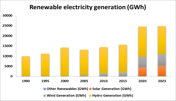
The Human Development Index (HDI) serves as a measure of inclusive growth. REN refers to Renewable energy consumption which measured as the total consumption of all renewable energy sources, including hydropower, solid biofuels, wind energy, solar energy, liquid biofuels, biogas, geothermal energy, marine energy, and energy from waste, and is expressed in terajoules (TJ), while NON_REN refers to the total energy consumption from non-renewable sources in terajoules (TJ).
ROL refers to the rule of law index that falls between 2.5 and -2.5, where 2.5 indicates a high level of respect for the rule of law, meaning the country has a strong judicial system, and laws are effectively enforced with respect for the rights of individuals and institutions, while -2.5 indicates a weak rule of law, meaning there are significant issues with the judicial system, little adherence to laws, and possibly corruption and instability of the legal system. TRD refers to the total foreign trade of exports and imports as a percentage of GDP. D1 and D2 are dummy variables. D1 reflects the social repercussions of the January 2011 revolution on the level of human development, while D2 reflects the impact of the Egyptian government's economic reform policies on the level of human development.
The model is based on annual data covering the period from 1990 to 2024, obtained from reliable sources such as the World Bank database and the United Nations Development Programme (UNDP) as shown in
Table 1. The Autoregressive Distributed Lag (ARDL) model was chosen due to its flexibility in dealing with non-integrated variables, its ability to be used to analyse both short and long term relationships, its incorporation of a bounds test to determine the existence of a long term equilibrium relationship, and an error correction model (ECM) to measure the speed of adjustment towards this equilibrium after the occurrence of shocks. This theoretical and measurement structure enables testing the main research hypothesis that renewable energy consumption can effectively contribute to promoting inclusive growth in Egypt, provided there is a supportive institutional environment and balanced trade policies.
Table 1. Data description and its sources.
Variables | Definition | Sources |
HDI | The Human Development Index | UNDP_Human Development Data Center |
REN | Renewable energy consumption (TJ) | World Bank, SE4All Database |
NON-REN | the total energy consumption from non-renewable sources (TJ) | World Bank, SE4All Database |
TRD | Trade (%GDP) | World Bank, (WDI) database |
ROL | the rule of law: estimation | World Bank, (WDI) database |
D1 | A dummy variable that expresses the social repercussions of the January 2011 revolution that takes only two values, 0 and 1 | Authors' creation depending on the nature of the dummy variables |
D2 | A dummy variable that expresses the impact of the Egyptian government's economic reform policies that takes only two values, 0 and 1 | Authors' creation depending on the nature of the dummy variables |
Source: Authors’ compilation
4. Methodology and Estimation Results
4.1. Estimation Methods
The model was estimated using the Augmented ARDL methodology, as this model allows the inclusion of variables with different lags based on model selection criteria such as the Akaike Information Criterion (AIC), which enhances the accuracy of the estimates. In addition, the Error Correction Model (ECM - Error Correction Model) was used to determine the speed of adjustment of the model from short-term imbalances towards long-term equilibrium
| [31] | Nkoro, E., & Uko, A. K. (2016). Autoregressive Distributed Lag (ARDL) cointegration technique: application and interpretation. Journal of Statistical and Econometric methods, 5(4), 63-91. |
[31]
.
To assess the quality of the model, a set of diagnostic tests were performed, including Breusch-Godfrey test to detect the presence of autocorrelation between errors, Breusch-Pagan-Godfrey test to check for heteroskedasticity, Jarque-Bera test to check that the probability distribution of the residuals follows a normal distribution and CUSUM test and Squares of CUSUM test to ensure that the parameters are stable over time. This methodology ensures that the model estimates are reliable and able to explain the economic relationships between variables, taking into account structural stability and ensuring that there are no econometric issues that may affect the accuracy of the results
| [32] | Gujarati, D. N., & Porter, D. C. (2009). Basic Econometrics (5th ed.). McGraw-Hill/Irwin. |
[32]
.
4.2. Estimation Results for Egypt
4.2.1. Results of Augmented ARDL Model
Table 2 shows the results of estimating a standard model based on temporal data, using variables recorded in logarithmic form. The dependent variable is the Human Development Index (LnHDI). The inclusion of LnHDI(-1) indicates that the model takes the form of a restricted autoregressive model with lagged variables. The model was estimated by classical linear regression, and the presented values indicate the coefficients of the variables, standard deviations, t-statistics, and their probabilities (P-values).
The first thing that stands out is the very high value of the coefficient of determination (R-squared = 0.999001), indicating that the model explains approximately 99.9% of the variance in the dependent variable. Although this value suggests a high fit of the model, its excessively high value may raise doubts about the possibility of an overfitting issue, especially when using temporal data that may contain autocorrelation. However, the value of the Durbin-Watson statistic (2.125) indicates the absence of autocorrelation of the residuals, reinforcing the reliability of the results in this respect.
The coefficient of LnHDI(-1) is 0.831062 and is statistically significant (P = 0.0000), meaning that the HDI in previous periods has a positive and significant impact on its current level, which is logically consistent with the cumulative nature of this indicator. This reflects that the change in human development does not occur suddenly, but is influenced by previous historical trends.
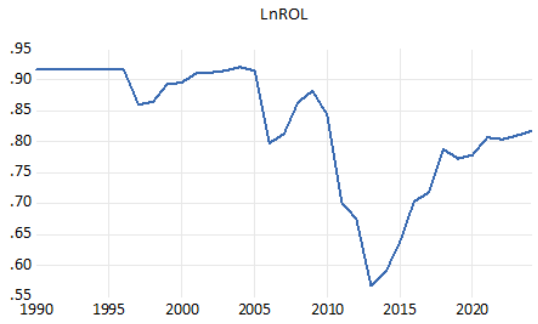
As for the renewable and non-renewable energy variables, the coefficients of LNREN and LnREN(-1) are positive but not statistically significant (P = 0.2389 and 0.2004, respectively), indicating that the contribution of renewable energy in improving the HDI is not strong or certain during the period under study. In contrast, non-renewable energy (LnNON_REN) is positively and statistically significant (P = 0.0005) with human development, which may reflect the study countries' greater reliance on traditional energy sources to enhance the well-being of the population, perhaps due to their availability or poor clean energy infrastructure. On the other hand, the rule of law (LnROL1) in its immediate form was not significant (P = 0.5223), but its lagged variable (LnROL(-1)) was negative and statistically significant (P = 0.0027). This suggests that improved rule of law indicators may have a delayed and negative impact on human development in the short term, which may be related to the effects of legal reforms on the redistribution of resources or the reduction of some rent-seeking practices.
Trade (LnTRD) was the most prominent variable with a negative and statistically significant effect in the current period (P = 0.0006), which may reflect that trade openness, if not accompanied by supportive social and economic policies, may lead to the marginalisation of certain segments of the population and negatively affect human development. While the lagged effect of trade (LnTRD(-1)) was positive but at the acceptable level of significance (P = 0.0945), which may indicate the existence of positive effects of trade in the medium or long term.
For D1, it was not significant (P = 0.5417), while D2 was positive and significant (P = 0.0057), indicating that there is a significant positive effect of this specific period on containment growth. In terms of model quality, the low negative values of the information criteria (Akaike, Schwarz, Hannan-Quinn) reflect a strong model fit with appropriate complexity. The low standard error of regression (S.E. of regression = 0.002833) also enhances the accuracy of the estimates.
Based on the above, it is clear that the estimated model provides a deep and coherent explanation of the factors influencing human development, but it also suggests that some positively hypothesised policies (such as renewable energy or trade) may not come to fruition directly or immediately, and that the effects depend on the temporal and institutional context of the country. These findings highlight the importance of designing comprehensive policies that take into account the delayed impact of certain variables, and not relying on one-dimensional models when pursuing inclusive growth.
Table 2. Results of Augmented ARDL Model.
Method: ARDL
Dependent Variable: LnHDI
Variable | Coefficient | Std. Error | t-Statistic | Prob.* |
LnHDI(-1) | 0.831062 | 0.032833 | 25.31178 | 0.0000 |
LnREN | 0.021430 | 0.017745 | 1.207668 | 0.2389 |
LnREN(-1) | 0.024396 | 0.018528 | 1.316688 | 0.2004 |
LnNON_REN | 1.720426 | 0.430516 | 3.996196 | 0.0005 |
LnROL | -0.011425 | 0.017596 | -0.649296 | 0.5223 |
LnROL(-1) | -0.042683 | 0.012765 | -3.343634 | 0.0027 |
LnTRD | -1.832065 | 0.460153 | -3.981422 | 0.0006 |
LnTRD(-1) | 0.007668 | 0.004405 | 1.740960 | 0.0945 |
D1 | -0.002268 | 0.003664 | -0.619122 | 0.5417 |
D2 | 0.009570 | 0.003154 | 3.034594 | 0.0057 |
4.2.2. Results of Augmented ARDL Diagnostic Tests
To evaluate the quality of the Augmented ARDL model, four diagnostic tests were performed as follow: the Breusch-Pagan-Godfrey test, the Breusch-Godfrey Serial Correlation LM test, the Histogram-Normality test, and the Optimal Lag Length Selection test. These tests are important steps before performing the Augmented ARDL Bound test.
Table 3 presents the results of the heteroskedasticity test using the Breusch-Pagan-Godfrey test, which is one of the most prominent tests used in econometrics to detect the persistence of error variance in a regression model. In its null hypothesis, the test assumes homoskedasticity, meaning that the variance of the random components remains constant across all observations, while the alternative hypothesis suggests the presence of heteroskedasticity, which violates the assumptions of the classical model and may lead to inefficient estimation and faulty statistical inference.
The test results indicate that the F statistic is (0.6939) with a p-value of (0.7201), meaning that this test cannot reject the null hypothesis at any conventional significance level (such as 1%, 5%, or even 10%). This is replicated in the rest of the accompanying statistics: The Obs*R-squared statistic (7.8805) was associated with a probability value of 0.6405, as was the Scaled Explained Sum of Squares statistic with a probability value of 0.7395. All these results indicate a high degree of consistency in the conclusion that there is no statistical evidence to support the hypothesis of the existence of variable variance in the residuals. This result strengthens the reliability of the estimates presented in the original model, especially since one of the most important conditions for the efficiency of the OLS estimator is the stability of the variance of the random components. A variable variance would have meant that the estimators remain unbiased but become inefficient, and the hypothesis testing associated with the model coefficients would have been invalid. Refuting the alternative hypothesis (i.e., accepting the homogeneity hypothesis) gives the researcher additional confidence in the accuracy and completeness of the estimated model properties.
It is worth noting that the use of the Breusch-Pagan-Godfrey test, which is based on the least squares analysis of the squared error of the residuals, is an appropriate methodological choice in this context, especially in models with a relatively large number of explanatory variables, as is the case in the model under study. The choice of this test also reflects a scientific awareness of the potential for covariance to affect the reliability of the results, especially in complex temporal models..
Table 3. Results of Breusch-Pagan-Godfrey test.
Heteroskedasticity Test: Breusch-Pagan-Godfrey Null hypothesis: Homoskedasticity |
F-statistic | 0.693929 | Prob. F(10,23) | 0.7201 |
Obs*R-squared | 7.880475 | Prob. Chi Square(10) | 0.6405 |
Scaled explained SS | 6.849903 | Prob. Chi-Square(10) | 0.7395 |
Table 4 presents the results of the Breusch-Godfrey LM Test to detect autocorrelation in the residuals up to the second term (lag 2), a test widely used in econometrics to check whether one of the basic assumptions in classical linear regression models is violated, namely that there is no serial correlation between the errors. The importance of this test lies in its ability to handle models with lagged variables, unlike the traditional Durbin-Watson test which may give misleading results in such cases. The null hypothesis of the Breusch-Godfrey test assumes that there is no autocorrelation in the residuals up to the second order, i.e. that the random components of the model are independent over time. The alternative hypothesis states that there is at least first- or second-order autocorrelation, which can lead to inefficient estimates and make statistical hypothesis tests susceptible to bias.
The presented results indicate that the F statistic reached (1.1769), which is associated with a probability value (p-value) of (0.3269), while the Obs*R-squared statistic reached (3.2862) with a probability value of (0.1934). These values indicate that the null hypothesis cannot be rejected at any conventional significance level (1%, 5%, or even 10%). Consequently, the model is free of autocorrelation within the limits tested. The absence of autocorrelation in the residuals is a pivotal result in assessing the quality of the standard model, because serial correlation means that the residuals contain information not captured by the independent variables, which violates the assumption of randomness and leads to unreliable estimates. In contrast, this result confirms that the model is able to explain the phenomenon under study without the temporal data leaving an unexplained effect in the errors.
Methodologically, the adoption of the Breusch-Godfrey test instead of simpler tests reflects the researcher's keenness to adhere strictly to the strictest standardisation criteria, especially as it allows the possibility of examining higher order autocorrelation, which is crucial when dealing with time-series data containing dynamic or lagged components.
Table 4. Results of Breusch-Godfrey Serial Correlation LM Test.
Breusch-Godfrey Serial Correlation LM Test Null hypothesis: No serial correlation at up to 2 lags |
F-statistic | 1.176947 | Prob. F(2,22) | 0.3269 |
Obs*R-squared | 3.286225 | Prob. Chi-Square(2) | 0.1934 |
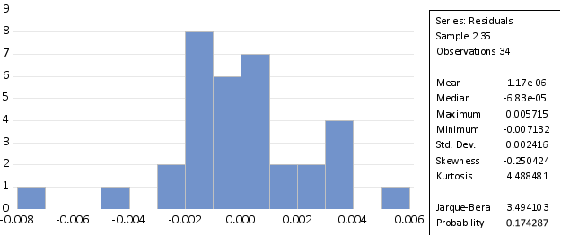
Figure 1 and the accompanying statistical analysis reflect an assessment of the residuals characteristics of the estimated standard model, which is necessary to ensure the validity of the basic assumptions of the Ordinary Least Squares (OLS) method, in particular the assumption of a normal distribution of residuals. Examining the residuals is a pivotal step to check the fit of the model, as many statistical tests (such as hypothesis tests for coefficients) rely on the assumption that errors follow a normal distribution.
The statistical analysis indicates that the mean residuals are very close to zero (-1.17e-06), and the median is also close to zero (-6.83e-05), indicating that the distribution of residuals is centered around zero, consistent with the properties of a normal distribution. The standard deviation (Std. Dev.), which is about 0.002416, indicates that the dispersion of the residuals is relatively limited, enhancing confidence in the accuracy of the estimates. On the other hand, the Skewness value of -0.250424 indicates that the residual distribution is slightly skewed towards the left side (negative), but this skew is very limited and does not represent a significant deviation from symmetry. The Kurtosis, with a value of 4.484481, is higher than the ideal value for a normal distribution (3), indicating a more Leptokurtic distribution, i.e. there is a greater concentration of observations around the mean with slightly longer tails than a normal Gaussian distribution.
The Jarque-Bera test, a common test for detecting deviation from normality based on skewness and kurtosis, yielded a statistical value of 3.494103 with a probability value of 0.174287. Since the probability value is higher than conventional significance levels (such as 0.01, 0.05, or even 0.10), the null hypothesis that the residues follow a normal distribution cannot be rejected. Thus, it is possible to conclude that the residuals do not suffer from intrinsic distributional issues. The histogram supports this analysis, showing a distribution of residuals centered around zero, with a distribution that closely approximates the typical bell-shape of a normal distribution, although there are some slight deviations on the edges, which do not seem alarming given the relative sample size (34 observations).
Figure 1. Results of HISTOGRAM-NORMALITY TEST.
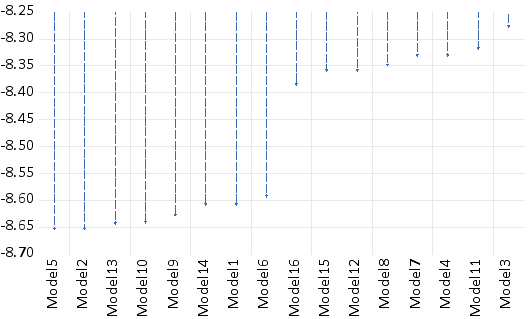
Figure 2 shows a comparison of a set of models estimated according to the Akaike Information Criterion (AIC), which is one of the most common criteria in econometrics for choosing the optimal model. Akaike's criterion is based on balancing the goodness of fit with the number of estimated parameters, rewarding models that achieve a good explanation of the data with the fewest number of parameters, thereby minimizing the issue of overfitting. In theory, the lower the AIC value, the better the model. It can be clearly seen from the figure that Model5 has the lowest AIC value compared to the rest of the models, indicating that it is the best fitting model. This is closely followed by Model2 and Model12, which show significantly lower values, but not as low as Model5. It is important to note that small differences in AIC values may not necessarily be significant in practice, but the large difference as observed between the first and last models indicates a clear superiority.
This choice is reinforced by the fact that Akaike's criterion considers the sample size and the number of parameters in balance, which means that the chosen model not only achieves the best fit to the data, but also avoids redundant model complexity. It can be seen from the bottom menu of the graph that each model is defined by a specific structure (defined by the order of delays for the different variables), indicating that the research has systematically compared multiple configurations of ARDL models.
Figure 2 also reflects the rigorous scientific method used to select the model, as a wide variety of models were tested and no single model was directly relied upon, lending strong credibility to the entire research process.
Figure 2. Akaike Information Criterion.
4.2.3. Results of Augmented ARDL Bound Test
To determine whether there is cointegration or not and to to understand the nature of this relationship in the long run, the following tests were performed: Overall F-Bounds Test, t-Bounds Test, Exogenous F-Bounds Test as an essential part of. In a subsequent step, structural stability tests of the model parameters (CUSUM Test and Squares of CUSUM test) were performed to ensure that there is no structural change in the data that would lead to an error in the stability and consistency of the short-term model parameters with the long-term model parameters.
Table 5 presents the results of the F-Bounds Test under the ARDL methodology, which is an advanced analytical technique used to examine the existence of a long-run equilibrium relationship between variables, even if these variables are a combination of I(0) and I(1) integration levels, provided they are not I(2). The aim of the boundary test is to resolve the issue of cointegration between variables without having to examine the unit root characteristics of each variable separately. The null hypothesis of this test states that there is no long-run relationship between the variables, that is, the dependent variable is not cointegrated with the independent variables in the long run. The alternative hypothesis states that there is a long-run equilibrium relationship, which is a necessary condition for changes in the dependent variable (usually a central economic or social indicator) to be explained by the other variables.
The results of the table indicate that the F statistic value is (33.19064), which is significantly higher than the critical values defined by Pesaran, Shin, and Smith, which are usually used as a benchmark for this type of test. These critical values vary according to the levels of significance (1%, 2.5%, 5%, 10%) and according to whether the variables are dependent on a zero-degree integration (I(0)) or first order (I(1)). At the 5% significance level, for example, the limits lie between 2.26 (for I(0)) and 3.48 (for I(1)), which means that any value of the F statistic that exceeds the upper limit (I(1)) allows the null hypothesis to be rejected in favour of the alternative hypothesis.
Since the calculated value (33.19064) significantly exceeds even the highest critical value at the 1% significance level (4.44), the result is clear and conclusive: There is a long-run equilibrium relationship between the dependent variable and the independent variables in the model. This result carries great theoretical and practical significance, as it indicates that the independent variables do not only affect the dependent variable in a momentary or instantaneous manner, but also have a deep relationship with it that extends over the long term, which strengthens the causal interpretation of the model and gives it strong analytical legitimacy.
Interestingly, the sample size used in this estimation is (34), which is a relatively small sample, which is reflected in the absence of finite sample critical values in the table. However, the very high value of the F statistic exceeds even what might be expected in larger samples, making the result statistically robust despite the limited sample size.
Table 5. Results of Augmented ARDL Bound Test.
Overall F-Bounds Test
Null Hypothesis: No levels relationship
Test Statistic | Value | Signif. | I(0) | I(1) |
| | | Asymptotic: n=1000 | |
F-statistic | 33.19064 | 10% | 1.9 | |
K | 4 | 5% | 2.26 | |
| | 2.5% | 2.62 | |
| | 1% | 3.07 | |
Actual Sample Size | 34 | | Finite Sample: n=35 | |
| | 10% | -1 | |
| | 5% | -1 | |
| | 1% | -1 | |
| | | Finite Sample: n=30 | |
Table 6 shows the results of the t-test, which is a complementary test to the F-test within the ARDL methodology developed by Pesaran et al.
| [33] | Pesaran, M. H., & Shin, Y. (1995). An autoregressive distributed lag modelling approach to cointegration analysis (Vol. 9514, pp. 371-413). Cambridge, UK: Department of Applied Economics, University of Cambridge. |
[33]
This test is specifically used to assess the existence of a long-run equilibrium relationship between the variables by examining the significance of the lagged level of the dependent variable. The t-test is a flexible way to test the null hypothesis that there is no long-term relationship between the variables under study. The calculated value of the t-statistic is -5.145370, which is a negative value that is high in strength and reflects a steep downward trend. When compared to the critical values at different significance levels, it is clear that this value falls outside both the lower and upper limits. At the 5% significance level, for example, the critical values lie between -1.95 (for I(0) variables) and -3.6 (for I(1) variables), while the calculated value (-5.145) is well below the upper limit of -3.6. This pattern is repeated at all other significance levels, including the most stringent one (1%), where the upper bound is -4.23, which is still lower in absolute value than the actual value of the test.
This result is interpreted as providing strong evidence to reject the null hypothesis that denies the existence of a long-term relationship between the variables. Thus, the dependent variable shows a statistically significant equilibrium correlation with the independent variables in the long run, which reinforces the validity of the dynamic model used, and provides scientific justification for completing the analysis by decomposing the relationships into short and long term components within the full ARDL model. The statistical power of this result is increased by the fact that the t-test is more conservative than the F-test, as it directly tests the Error Correction Term. Thus, the fact that the calculated value exceeds all critical limits strongly enhances the reliability of the results and shows that the relationship between the variables is not casual or instantaneous, but rather governed by a stable and long-term dynamic.
From an econometric point of view, this result is an indicator of the gravitational property of the dynamic system of the relationship, which means that any deviation from equilibrium in the current period will be gradually corrected in future periods, which is the essence of the idea of a long-term equilibrium relationship. The results of the t-bounds test are a crucial support for the robustness of the theoretical and parametric model adopted in the study, and represent an essential pillar in building an integrated analysis that accurately distinguishes between instantaneous and cumulative effects, and paves the way to proceed to estimating the error correction model (ECM) to elucidate the short-term dynamics within a framework consistent with the verified equilibrium relationship.
Table 6. Results of t-Bounds Test.
t-Bounds Test
Null Hypothesis: No levels relationship
Test Statistic | Value | Signif. | I(0) | I(1) |
t-statistic | -5.145370 | 10% | -1.62 | -3.26 |
| | 5% | -1.95 | -3.6 |
| | 2.5% | -2.24 | -3.89 |
| | 1% | -2.58 | -4.23 |
Table 7 shows the results of the Exogenous F-Bounds Test, which is used within the framework of the extended ARDL methodology to assess the existence of a long-run equilibrium relationship, but with a focus on the relationship of the dependent variable with exogenous variables specifically, i.e. those that are assumed to be unaffected by the dependent variable within the standard model used. This approach differs from the traditional F-Bounds test in that the relationships examined here relate exclusively to directional links from the explanatory variables to the dependent variable, without the complexities of mutual interaction between the variables.
The null hypothesis of the test states that there is no level relationship between the exogenous variables and the dependent variable, meaning the absence of any form of long-run equilibrium relationship, while the alternative hypothesis indicates a long-run causal association between the exogenous variables and the explanatory variable. The results of the table indicate that the calculated F statistic is 9.548276, which is a very high value. When compared to the critical values both in the asymptotic case of a large sample (n=1000) and in the case of a small sample (n=34), we find that this value exceeds all upper limits (I(1)) at all significance levels, including the most stringent one (at the 1% level), where the upper limit for the small sample (n=35) is about 6.33, while the calculated value exceeds this and reaches 9.548.
The fact that the calculated value exceeds this upper bound by a large margin provides conclusive evidence to reject the null hypothesis and accept the existence of a long-run equilibrium relationship between the dependent variable and the exogenous variables. This statistical finding is particularly important in models that aim to analyze the causal impact of external economic policies or variables (such as trade, investment, energy, or governance) on complex indicators such as growth, human development, or financial stability. The strength of this result shows that the estimated model not only suffers from the absence of spurious correlation bias, but also shows that the relationship between the exogenous variables and the dependent variable is a stable structural relationship. Theoretically, the existence of this relationship is a confirmation that the dependent variable responds systematically to changes in its determinants, which enhances the credibility of the estimates both in an academic context and in applied decision-making frameworks.
In conclusion, the results of the Exogenous F-Bounds test clearly indicate that the identified explanatory variables are long-term causal determinants of the dependent variable, which lends the model high explanatory power and theoretical legitimacy, and provides a transitional basis towards ECM analysis and the interpretation of short-term interactions in light of the verified general equilibrium.
Table 7. Results of Exogenous F-Bounds Test.
Exogenous F-Bounds Test
Null Hypothesis: No exo. levels relationship
Test Statistic | Value | Signif. | I(0) | I(1) |
| | | Asymptotic: n=1000 | |
F-statistic | 9.548276 | 10% | 1.95 | 3.46 |
K | 4 | 5% | 2.39 | 4.01 |
| | 2.5% | 2.82 | 4.57 |
| | 1% | 3.37 | 5.35 |
Actual Sample Size | 34 | | Finite Sample: n=30 | |
| | 10% | 2.18 | 3.78 |
| | 5% | 2.75 | 4.61 |
| | 2.5% | 3.34 | 5.46 |
| | 1% | 4.13 | 6.67 |
| | | Finite Sample: n=35 | |
| | 10% | 2.15 | 3.76 |
| | 5% | 2.71 | 4.54 |
| | 2.5% | 3.27 | 5.31 |
| | 1% | 4.04 | 6.33 |
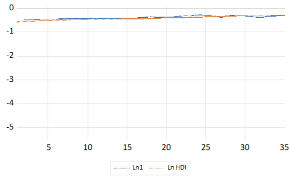
To illustrate whether the logical cointegration relationship is normal or degraded,
Figure 3 presents a time comparison between two variables, Ln1 and Ln HDI, across 34 time points. It can be seen from the plot that the two series move very closely together, with values centered in a narrow range close to zero, with very slight differences. The logical co-integration relationship is therefore normal (not degraded).
Figure 3. Graphical Comparison of Actual and Fitted Values.
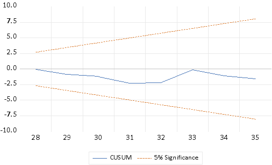
Figure 4 presents the result of the CUSUM test, a commonly used test to assess the stability of model parameters over time, especially in time series and ARDL autoregressive models. The goal of this test is to check whether the model parameters remain constant over the study period, or whether there are Structural Breaks that affect the stability of the estimated relationships. In this figure, the blue line represents the trajectory of the CUSUM statistic over time, while the red lines represent the confidence interval limits at the 5% significance level. It is clear that the path of the cumulative residuals of the successive estimation of the model parameters (blue line) is centered on the path of the upper and lower bounds (red lines) and did not go outside the range of the bounds (upper and lower), thus this is an indication that the model parameters are stable, which is a good and desirable characteristic of the model, which means there is structural stability of the model parameters.
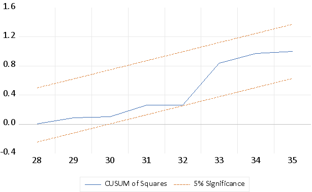
Figure 5 represents the result of the CUSUM of Squares test, another important test used to evaluate the stability of residual variance and model coefficients over time. Different from the regular CUSUM test that only measures the stability of the coefficients, CUSUM of Squares focuses specifically on fluctuations or sudden changes in error variance, making it sensitive to major structural shifts that may not show up with a simple CUSUM test. In the figure, the blue line represents the CUSUM of Squares statistical path, while the red lines represent the confidence interval limits at the 5% significance level. From the above, it is clear that the cumulative sum of squares of the residuals of the model (blue line) is centered on the path of the upper and lower bounds (red lines) and does not deviate from the range of the upper and lower bounds. This is an indication that the model parameters are stable, which is a good and desirable characteristic of the model.
Figure 5. CUSUM of Squares Test.
4.2.4. Results of Estimating Long-term Parameters
The results of
Table 8 reflect the estimation of the levels equation within the autoregressive distributed lag (ARDL) model in Case 1: No Constant and No Trend, which is an analytical formula used when variables are assumed to be correlated without a fixed underlying level of the relationship or a general time trend. This estimation aims to reveal the long-term equilibrium relationship between inclusive growth (Ln HDI) and a set of important economic and institutional variables, namely: Renewable Energy (LnREN), Non-Renewable Energy (LnNON_REN), Rule of Law (LnROL), and Trade Openness (LnTRD).
The results indicate a strong and statistically significant long-run correlation between the dependent variable and the four independent variables, as all estimated coefficients are significant at the 1% significance level, and high t-statistics reflect a high level of confidence in the validity of the estimate. The renewable energy coefficient (LnREN), which reached 0.271258, shows that increased reliance on clean energy is associated with an improvement in inclusive growth, which is consistent with recent literature that emphasizes the role of sustainable energy sources in supporting the well-being of societies, by reducing emissions and improving quality of life.
The non-renewable energy coefficient (LnNON_REN) was significantly high (10.18377), which indicates a high dependence on these sources in supporting the economic and social structure in the studied countries. This may be because economies that rely on the extraction and export of fossil resources such as oil and gas generate significant revenues that are used to improve public services and infrastructure, reflecting positively on education, health and income indicators, which are key components of the Human Development Index (HDI). However, this positive impact is not without risks, as it may reflect what is known as "resource-contingent development," which shows positive results in the short term without ensuring sustainability in light of global market fluctuations.
In contrast, the results show that the rule of law (LnROL) is negatively associated with inclusive growth in the long run, with a coefficient of -0.320284. This estimate, while statistically significant, requires careful interpretation, as it may indicate that improvements in the legal framework only pay off in the long run or are associated with reform measures that may create transitional effects that temporarily reduce services or redirect resources. This could also be a reflection of the disconnect between implementation and theorizing, where legal reforms are implemented that do not necessarily lead to a direct improvement in individual well-being in the absence of effective implementing institutions.
Figure 6 shows the behavior of the variable (LnROL) in the long run.
On the other hand, the coefficient of trade openness (LnTRD) shows a negative and strong effect (-10.79921), which is of scientific interest, as it is assumed in the classical economic literature that openness to trade promotes growth and provides greater opportunities for social welfare. However, this result suggests that, in the studied context, trade may have contributed to widening development gaps rather than reducing them, perhaps due to unequal competition, the weak capacity of the domestic economy to absorb external shocks, or the absence of social protection policies that counterbalance the negative effects of trade liberalization. This result may also reflect an over-reliance on imports or weak domestic value-added in global production chains.
Figure 7 shows the behavior of the variable (LnTRD) in the long run.
The table concludes with the error correction equation that forms the core of the long-term equilibrium relationship, where the structural equilibrium between the variables is represented in an explicitly linear form. This equation is the basis for a short-term dynamical model (ECM), which aims to determine how quickly the system responds to any shock or deviation from equilibrium.
Table 8. Results of estimating long-term parameters.
Method: ARDL (Autoregressive Distributed Lag), Case 1: No Constant and No Trend
Dependent variable: LnHDI
Variable | Coefficient | Std. Error | t-Statistic | Prob. |
LnREN | 0.271258 | 0.033802 | 8.024929 | 0.0000 |
LnNON_REN | 10.18377 | 1.189107 | 8.564218 | 0.0000 |
LnROL | -0.320284 | 0.079092 | -4.049535 | 0.0005 |
LnTRD | -10.79921 | 1.267768 | -8.518286 | 0.0000 |
Figure 6. Long-term Trend of The Variable LnROL.
4.2.5. Results of ECM Regression
Table 9 reflects the results of estimating the Error Correction Model (ECM) in the context of the selected ARDL model, which is used to analyse the short-term dynamic relationship between the variables, in the presence of a long-term equilibrium relationship previously verified by Bounds Tests. The model is based on the ARDL (1, 1, 1, 0, 1, 1, 1) formula, which means that the dependent variable, the change in inclusive growth (D (Ln HDI)), is influenced by its lagged values and independent variables including renewable energy, rule of law, trade, as well as two dummy variables D1 and D2, without including a constant term or time trend, in line with the specific case of the model (No Constant and No Trend).
The results of the model show that the error correction coefficient (CointEq (-1)) was negative and very statistically significant (p < 0.0001), with a value of -0.168938. This value represents the core of the model, indicating the proportion of adjustment the system makes towards the long-run equilibrium in each period. In other words, about 17% of the deviation from the equilibrium relationship is corrected in the subsequent period, which reflects a moderate speed of adjustment towards equilibrium and confirms the existence of a stable dynamic of the studied economic system.
Looking at the explanatory variables in the short term, we find that the only variable that retained strong statistical significance is the change in trade openness (D(Ln TRD)), with an impact coefficient of -1.832065 and a t-statistic of -13.89, which indicates a rapid and strong negative impact of the change in trade on human development in the short term. This result is of great analytical importance, as it shows that trade shocks sharply affect social welfare indicators if they are not offset by social protection policies or capacity enhancement.
The rest of the variables, such as the change in renewable energy (D(LnREN)) or rule of law (D(LnROL)) were not statistically significant, although their coefficients took the same direction as the long-term relationship, reflecting that their impact needs time to crystallise within the general equilibrium. The variables D1 and D2 showed a differential effect; D1 was not significant, while D2 had a positive and significant effect on human development, reflecting the impact of economic reform policies on inclusive growth.
Measures of model quality indicate a relatively good fit, with a coefficient of determination R-squared of 0.697, meaning that approximately 70% of the short-term change in the HDI can be explained by the variables included in the model. The value of the Durbin-Watson statistic (2.125) indicates the absence of autocorrelation in the residuals, which enhances confidence in the validity of the estimation. The information criteria (Akaike, Schwarz, Hannan-Quinn) show low levels, which is a positive indication of the quality of the model and its superiority over more complex alternative models.
The importance of this model lies not only in explaining the instantaneous changes of the CGI, but also in its ability to systematically link short-term dynamic analysis with long-term structural equilibrium. It shows how momentary shocks interact with the structural structure of the system and provides a powerful tool for decision-makers to assess the sustainability of economic and social policies.
Table 9. Results of ECM Regression.
Method: ARDL Error Correction Regression (ECM), Case 1: No Constant and No Trend
Dependent Variable: D(LnHDI)
Variable | Coefficient | Std. Error | t-Statistic | Prob. |
D(LnREN) | 0.021430 | 0.014816 | 1.446369 | 0.1610 |
D(LnROL1) | -0.011425 | 0.011187 | -1.021319 | 0.3173 |
D(LnTRD) | -1.832065 | 0.131867 | -13.89328 | 0.0000 |
D1 | -0.002268 | 0.001485 | -1.527045 | 0.1398 |
D2 | 0.009570 | 0.001913 | 5.002328 | 0.0000 |
CointEq(-1)* | -0.168938 | 0.012141 | -13.91446 | 0.0000 |
4.2.6. Results of Forecast Evaluation Test
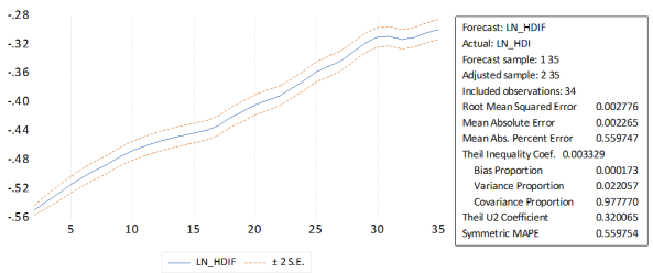
Figure 8 displays the Forecast Evaluation, which shows a comparison between the actual values of LnHDI and the predicted values of LnHDI, with confidence intervals of ±2 standard deviations (±2 S.E.). This type of analysis is very important for examining the predictive accuracy of the model, and is a necessary step to assess how reliable the model is not only in explaining in-sample data, but also in future predictions.
It can be seen from
Figure 8 that the predicted values follow the actual values very closely along the sample period, with most of the values staying within the confidence interval. This indicates that the model achieves good predictive performance without large deviations or typical errors. The forecast quality analysis sidebar displays a rich set of quantitative indicators that allow for accurate evaluation of model performance. The low Root Mean Squared Error (RMSE) value of 0.002776 indicates that the differences between the actual and predicted values are very small, reflecting the model's high forecast accuracy. The Mean Absolute Error (MAE) of 0.002265 supports this conclusion, confirming that absolute deviations from the true values are very limited.
On the other hand, the Mean Absolute Percent Error (MAPE) ratio, estimated at approximately 0.5597%, shows that the relative error of the forecasts is remarkably low, a strong indicator of the quality of the fit within the economic context. In the same vein, the Theil Inequality Coefficient (U) results, which recorded a value of 0.00339, reinforce the model's credibility. This low value indicates that the predictions significantly outperform random predictions, enhancing the reliability of the predictive results. Breaking down the components of the Theil error, the Bias Proportion of 0.000173 shows that the error resulting from bias in the estimates is almost nonexistent, reflecting the model's neutrality. The Variance Proportion of 0.02057 also indicates that the difference between the predictions and the actual values in the changes is very small, while the Covariance Proportion of 0.97777 demonstrates that the majority of the quality of the predictions is due to the strong correlation between the predicted and actual values, a crucial result in confirming the model's effectiveness.
The Theil U2 coefficient, which reached 0.032056, provides an additional measure of the quality of the estimate, as it also confirms the model's positive performance across another independent criterion. Finally, the symmetric relative absolute error (MAPE), estimated at 0.5597%, supports previous findings by taking into account the symmetry of errors, providing a more accurate assessment of the model's performance. Based on these combined indicators, it can be concluded that the model has a high ability to accurately and reliably predict future values, enhancing its suitability for use in economic analysis and policy forecasting.
Figure 8. Forecast Evaluation Metrics.