Research Article | | Peer-Reviewed

Forecasting the International Market Prices for Rice, Corn and Soybeans Using ARIMA Time Series Modelling

Received: 4 June 2025     Accepted: 16 June 2025     Published: 7 July 2025
Views:       Downloads:
Abstract

Rice, corn, and soybeans are among the most widely cultivated crops, making them crucial for global food security and the economic well-being of many countries. Like many other crops, the global prices for these commodities are prone to fluctuations due to unfavorable weather conditions, natural disasters (like flooding), global demand, and economic crises. Consequently, their prices are subject to significant changes and volatility. Forecasting and modelling these prices offer valuable insights to policymakers and local growers within the agricultural sector. While there is a plethora of studies focusing on forecasting prices based on data obtained for a specific locality, country, or region, there is a paucity of publications that take on a more global outlook for rice, corn, and soybeans. The objective of this study is to use an Autoregressive Integrated Moving Average (ARIMA) process to model and forecast the international market prices of milled rice (5% broken), corn, and soybeans. We relied on World Bank data covering the period from 1988 to 2018 to construct several time series models. The average prices for milled rice, corn, and soybeans are $344.47, $144.48, and $334.72 (USD) per metric ton, respectively. The results of the model selection procedure indicate that the ARIMA (5,1,4), ARIMA (6,1,3), and ARIMA (6,1,1) models best fit the prices of milled rice, corn, and soybeans, respectively. Furthermore, these models offer the best in-sample and out-of-sample performances. The accuracy of the projected values, derived from the chosen models, was evaluated by calculating several metrics, including the mean absolute error (MAE), mean squared error (MSE), root mean square error (RMSE), and mean absolute percentage error (MAPE). This paper highlights the utility and applicability of the ARIMA model as a powerful tool for forecasting agricultural prices. Our modeling framework could enable governments and agribusinesses to (a) better anticipate global price fluctuations, (b) optimize trade decisions, (c) strengthen food security planning, and (d) engage in more sustainable agriculture.

Published in International Journal of Agricultural Economics (Volume 10, Issue 4)
DOI 10.11648/j.ijae.20251004.13
Page(s) 170-182
Creative Commons

This is an Open Access article, distributed under the terms of the Creative Commons Attribution 4.0 International License (http://creativecommons.org/licenses/by/4.0/), which permits unrestricted use, distribution and reproduction in any medium or format, provided the original work is properly cited.

Copyright

Copyright © The Author(s), 2025. Published by Science Publishing Group

Keywords

ARIMA Model, Price Volatility, Time Series Forecasting, Rice, Corn, Soybean, Economic Modeling, Agricultural Commodities

1. Introduction
Rice, corn, and soybeans are primary staple foods and sources of calories, proteins, and essential nutrients for a large portion of the world's population. They significantly impact the economies of many nations and play a significant role in global food security. Additionally, these three crops have become increasingly crucial as industrial crops, with various applications in producing biofuels, animal feed, flour and several consumer products. Consequently, having insights into their future economic status will be vital for the global agricultural sector and overall food security.
The macroeconomic performances of the rice, corn, and soy industries, like many other industries, are significantly affected by price changes and fluctuations. Agricultural commodity prices inherently display volatility and dynamic variations over time as they consistently respond to various shifts . Such price volatility can profoundly impact production decisions, posing challenges for producers in accurately predicting future price levels and efficiently organizing sales . Producers with a risk-averse disposition may reduce their output in response to pricing uncertainty and, conversely, increase output when confronted with price certainty. This behavior has implications for the availability of food supplies . Consequently, accurate prediction of price changes is critical for formulating sound economic policies. It enables policymakers and farmers to ascertain the scale of sales and establish an appropriate strategy to optimize revenue from crop production.
Time series analysis is frequently employed for price forecasting. It uses historical price data to make inferences about the likely future prices. A widely used method for forecasting time series data is the Autoregressive Integrated Moving Average (ARIMA) modeling, which considers a time series' autocorrelation and moving average components to predict future values. This relies on understanding the intrinsic dynamic nature of prices shaped by various factors such as macroeconomic variables, the environment, and international trade . ARIMA models capture temporal dependencies that influence agricultural markets. These include seasonal effects associated with planting and harvesting patterns , external factors such as energy prices , and feedstock dynamics .
Its utility and applicability have led to numerous studies employing the ARIMA model to forecast crop prices of local and regional markets. These include paddy , rice , wheat , peas and vegetables , tomatoes, and soybeans . A common denominator for forecasting prices with ARIMA is the emphasis on accuracy and precision, achieved by aligning in-sample forecasts and actual out-of-sample evidence, and through additional processes, such as the Kalman filter technique, and seasonal ARIMA (SARIMA).
As price forecasting becomes increasingly essential in the global agricultural sector, this study aims to determine the best ARIMA time series model for forecasting the prices of milled rice, corn, and soybeans. While many studies focus on forecasting prices based on data obtained for a specific locality, country, or region, this paper adopts a more global outlook. This model forecasts monthly prices for rice (milled), corn, and soybeans per metric ton over a 12-month window. It utilizes monthly data from the World Bank database, spanning from 1988 to 2018. The significance of this study lies in its validation of the suitability and accuracy of the ARIMA model for these agricultural prices on a global scale.
2. Materials and Methods
The objective of this study is to forecast the international prices for milled rice (5% broken), corn, and soybeans based on The World Bank's monthly agricultural commodity prices data . The dataset consists of 372 observations, which were used to construct the model and evaluate its in-sample performance. Twelve additional observations (January 2019 - December 2019) were used for testing the model's out-of-sample performance. All analysis was done using the R forecast, tseries, and fpp2 packages.
The present study utilizes the Box-Jenkins (1970) forecasting model, commonly referred to as the ARIMA model. The ARIMA model is a forecasting technique that relies on historical time series data of the underlying variable . The model can be expressed as follows:
Let yt represent a discrete time series, assuming distinct values over a certain period. The AR (p) model, an extension of the autoregressive model, represents the Yt series. This is expressed as:
ARp:Yt=φ0+φ1Yt-1+φ2Yt-2++φpYt-p+εt.
where Yt is the response variable at time t. Yt-1,Yt-2Yt-p is the respective variables at different times with lags, φ0,φ1,φp are the coefficients, and εt is the error factor.
Similarly, the MA(q) model, an extension of the moving average model, can be defined as follows (Pradhan, 2012).
MA(q): Yt=μt+εt+δ1εt-1++δqεt-q+vt
where μt is the constant mean of the series, δ1δq are the coefficients of the estimated error term; εt is the error term.
Combining both models is called the ARIMA model, which has the general form:
Yt=φ0+φ1Yt-1+φ2Yt-2++φpYt-p+εt+δ1εt-1++δqεt-q+vt, and is often expressed in shortened notation form ARIMA (p,d,q). Here, p is the order of the non-seasonal autoregressive part. d is the number of differencing operations to remove trends and stabilize the mean of a time series; this technique transforms a non-stationary time series into a stationary one. q is the order of the non-seasonal moving average model.
2.1. Determination of Stationarity
Confirming that the underlying data demonstrates stationarity is crucial to constructing the ARIMA model. Non-stationary time series typically display statistical characteristics that fluctuate over time. Consequently, ensuring the data is stationary is significant in the context of model development. The assessment of data stationarity involved employing various techniques, including visualization of time series graphs, analysis of autocorrelation functions (ACF) and the partial autocorrelation function (PACF) diagrams, and the application of the Augmented Dickey-Fuller test.
2.2. Candidate Model Order Selection
The next step in the modelling process is the determination of d, p, and q. The order of d is determined by the number of times the series is differenced. The determination of AR and MA signatures involves the use of non-seasonal autocorrelation function (ACF) and partial autocorrelation function (PACF) plots . A theoretical autoregressive (AR) model with an order of p exhibits an autocorrelation function (ACF) that decays, and a partial autocorrelation function (PACF) that cuts off at lag p. Conversely, a theoretical moving average (MA) model with an order of q displays a PACF that decays, and an ACF that cuts off at lag q. The best candidate models are the ones that are parsimonious and exhibit the lowest Akaike information criterion (AIC) values that best fit the given data .
2.3. Forecasting
After selecting suitable models, predicted values will be generated for use in both in-sample and out-of-sample testing. This is done to assess the models' performance on both seen and unseen data. The accuracy of the projected values, derived from the chosen models, was evaluated by calculating several metrics, including the mean absolute error (MAE), mean squared error (MSE), root mean square error (RMSE), and mean absolute percentage error (MAPE) . Additionally, confidence intervals were computed to indicate the level of uncertainty associated with the forecast of the best-choice model.
MAE=1Tt=1Tyˆt-yt=1Tt=1Tet 
MSE=1Tt=1Tyˆt-yt2=1Tt=1Tet2
RMSE=1Tt=1Tyˆt-yt2=1Tt=1Tet2 
where yt is the actual observation, ŷt is the fitted or forecast value, and T is the sample size.
2.4. Choice of Appropriate Model
The optimal model selection among candidate models was determined by assessing both in-sample and out-of-sample testing metrics, complemented by low AIC.
2.5. Diagnostics
A diagnostic check is a procedure used to verify the residuals. The residuals obtained from the best choice model were examined to determine if they exhibit characteristics of a white noise series, namely being uncorrelated and having a mean of zero. This was accomplished by analyzing the autocorrelation function (ACF) and partial autocorrelation function (PACF) plots, as well as conducting the Ljung-Box statistic test .
3. Results
Table 1. Summary statistics of the price of rice, corn, and soybeans from the years 1988-2018.

Descriptive

Rice

Corn

Soybeans

Mean

344.466

144.876

334.715

Median

311.500

118.795

290.500

Std. Deviation

126.858

59.588

117.607

Minimum

163.750

75.270

183.000

Maximum

907.000

333.053

684.020

Table 1 above summarizes descriptive measures for rice, corn, and soybeans prices from January 1988 to December 2018. Mean prices over this period were rice at $344.466, corn at $144.876, and soybeans at $334.715. Median values for this period were slightly lower, suggesting potential skewness. The standard deviations, ranging from $59.588 (corn) to $126.858 (rice), indicate significant long-term price variability. The minimum and maximum price ranges were $163.750 to $907.000 for rice, $75.270 to $333.053 for corn, and $183.000 to $684.020 for soybeans.
3.1. Testing for Stationarity
As previously mentioned, the assessment of the stationarity of the time series prices for rice, corn, and soybeans data was conducted through graphical inspection of the time series graph, analysis of the ACF and PACF plots, and by utilizing the Augmented Dickey-Fuller test. The time series graph (Figure 1), ACF and PACF plots (Figure 2), and the results of the Dickey-Fuller test are presented below:
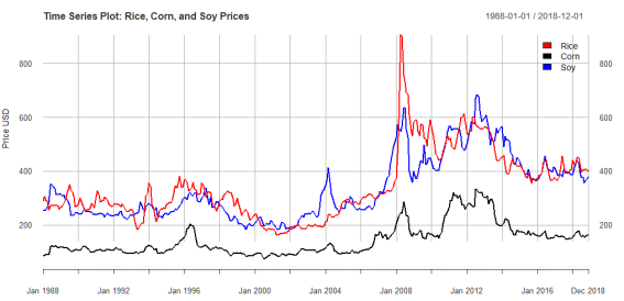
Figure 1. Time series plot of prices in USD for rice, corn, and soybeans (soy) from 1988-2018.
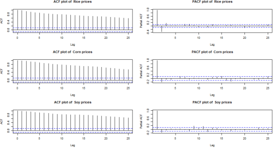
Figure 2. ACF and PACF plots of the prices of rice, corn, and soybeans (soy) from 1988-2018.
In Figure 1, we observed; price stability during periods (1988-2000) as the prices for rice, corn and soy exhibited moderate price fluctuations, a rising trends during the periods (2001-2007) being a gradual increase in prices, especially for rice and soy, a sharp spikes during the periods (2007-2008) observed in all three commodities prices with rice price experiencing the most dramatic surge peaking above USD 800, price volatility during the periods (2009-2014), and, stabilization and decline during the periods (2015-2018) as all three commodities trended downwards and stabilized (Rice and soybeans hovered near USD 400, while corn settled around USD 200).
The ACF and PACF plots of the prices of rice, corn, and soybeans can be seen in Figure 2. The results indicate non-stationarity of the prices of all three commodities. In the ACF plot, the lags decay slowly and remain above significance, suggesting the presence of unit roots.
3.1.1. Augmented Dickey-Fuller
To further conclude non stationarity of the data, an augmented Dickey-Fuller test was performed. The null hypothesis and results can be seen below.
Hypothesis of the Augmented Dickey-Fuller test
H0: The series has a unit root and is non-stationary.
H1: The series does not have a unit root. The series is stationary.
Augmented Dickey-Fuller Test with a set threshold of 0.05 for rice, corn, and soy
Dickey-Fuller =-2.1679, Lag order =7,p-value =0.5061 (Rice)
Dickey-Fuller = -2.4669, Lag order = 7, p-value = 0.3799 (corn)
Dickey-Fuller = -3.051, Lag order = 7, p-value = 0.1334 (Soybean)
The p-value for the Augmented Dickey-Fuller test performed on each commodity price exceeded 0.05 in all three instances, confirming that the data is indeed non-stationary and has unit roots.
3.1.2. Obtaining Stationarity
To make the data stationary, the technique of differencing was employed. If ' yt ' denotes the original series, the non-seasonal difference of first order is:
zt=yt-yt-1
After taking the first difference, the p-value of the Augmented Dickey-Fuller test was less than 0.01 for all three datasets, which is below the assumed level of significance of 0.05. This, along with the time series plots and ACF and PACF plots below, suggests that the first difference was sufficient to make the data stationary. Hence, the order of differencing, d, in the time series was taken to be equal to 1 (d=1).
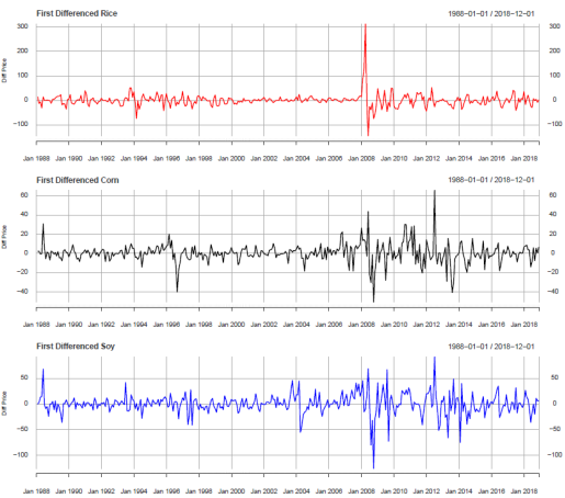
Figure 3. Time series plot of the first difference for rice, corn, and soybeans prices.
In Figure 3, it is observed that after differencing, the overall volatility is reduced, especially for rice and soybeans, which initially showed strong upward trends and sharp spikes. All three series exhibit mean-reverting behavior as they fluctuate more evenly around zero.
Augmented Dickey-Fuller Test
Dickey-Fuller =-8.747, Lag order =7,p-value <0.01 (rice)
Dickey-Fuller =-7.233, Lag order =7,p-value <0.01 (corn)
Dickey-Fuller =-7.676, Lag order =7,p-value <0.01 (Soybean)
The p-value for the Augmented Dickey-Fuller test performed on each commodity price after taking the first difference, are all less than 0.01 in all three instances, confirming that the data is now stationary and can be used in price forecasting.
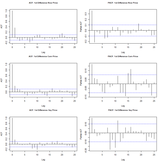
Figure 4. ACF and PACF plots of differenced prices of Rice, Corn, and Soybeans from 1988-2018.
The ACF and PACF plots of the differenced prices of rice, corn, and soybeans are shown in Figure 4. The results indicate that the prices of all three commodities are stationary. The ACF plots for each commodity exhibit a rapid decline to near-zero autocorrelations after the first few lags, indicating that the series no longer exhibit persistent trends or seasonality. The PACF plots show only significant spikes at the first or second lag, followed by negligible partial autocorrelations, suggesting that short-term relationships may exist, but long-term dependencies have been effectively removed.
3.2. Selecting the Best ARIMA Model for Forecasting
1) Candidate Model Order Selection
The ACF and PACF plots were used to determine the possible model orders. Lag Orders that made the model parsimonious were selected. Table 2 displays the selected candidate models, along with their corresponding AIC values.
Table 2. AIC values for selected models for rice, corn, and Soybean prices.

Rice

Corn

Soybean

Model

AIC

Model

AIC

Model

AIC

ARIMA(6,1,3)

3414.29

ARIMA(4,1,4)

2740.90

ARIMA(6,1,6)

3258.40

ARIMA(5,1,4)

3414.76

ARIMA(5,1,4)

2741.06

ARIMA(6,1,5)

3259.26

ARIMA(3,1,2)

3416.09

ARIMA(6,1,5)

2741.53

ARIMA(3,1,3)

3260.22

ARIMA(5,1,5)

3416.12

ARIMA(6,1,6)

2741.92

ARIMA(2,1,3)

3268.49

ARIMA(2,1,4)

3416.15

ARIMA(3,1,5)

2742.42

ARIMA(1,1,1)

3271.19

ARIMA(6,1,4)

3416.37

ARIMA(6,1,3)

2751.96

ARIMA(6,1,1)

3271.93

Based on Table 2, The best model based on the lowest AIC values are ARIMA(6,1,3) for rice prices, ARIMA(4,1,4) for corn prices and ARIMA(6,1,6) for soybean prices.
2) In-Sample Testing
Table 3, shows the in-sample performance of each selected model based on MAPE, MAE and RSME. Based on these results, ARIMA(6,1,3), ARIMA(6,1,5) and ARIMA(2,1,3) appear to be the best performing in sample model for rice, corn and soybean prices respectively.
Table 3. In-sample performance of rice, corn, and soybeans from 1988-2018.

Rice

Corn

Soybean

Model

MAPE

MAE

RMSE

Model

MAPE

MAE

RMSE

Model

MAPE

MAE

RMSE

ARIMA(6,1,3)

3.64

13.13

23.40

ARIMA(4,1,4)

4.00

6.09

9.46

ARIMA(6,1,6)

3.62

12.54

18.80

ARIMA(5,1,4)

3.67

13.19

23.19

ARIMA(5,1,4)

3.88

5.94

9.37

ARIMA(6,1,5)

3.61

12.58

18.87

ARIMA(3,1,2)

3.66

13.25

23.72

ARIMA(6,1,5)

3.84

5.88

9.32

ARIMA(3,1,3)

3.68

12.66

19.12

ARIMA(5,1,5)

3.67

13.18

23.40

ARIMA(6,1,6)

3.85

5.89

9.29

ARIMA(2,1,3)

3.60

12.50

19.46

ARIMA(2,1,4)

3.66

13.21

23.66

ARIMA(3,1,5)

3.88

5.99

9.46

ARIMA(1,1,1)

3.60

12.60

19.69

ARIMA(6,1,4)

3.67

13.19

23.41

ARIMA(6,1,3)

3.95

6.01

9.54

ARIMA(6,1,1)

3.63

12.65

19.44

3) Out-of-Sample Testing
Table 4 displays the performance of each model using unseen data from January 2019 to December 2019, based on MAPE, MAE, and RSME. Based on these results, ARIMA (5,1,4), ARIMA (6,1,3), and ARIMA (6,1,1) appear to be the best performing out-of-sample models for rice, corn, and soybean prices, respectively.
Table 4. Out-of-sample model performance for rice, corn, and soybeans from January 2019 - December 2019.

Rice

Corn

Soybean

Model

MAPE

MAE

RMSE

Model

MAPE

MAE

RMSE

Model

MAPE

MAE

RMSE

ARIMA(6,1,3)

3.099

13.100

15.596

ARIMA(4,1,4)

6.276

10.807

12.707

ARIMA(6,1,6)

6.163

22.307

25.421

ARIMA(5,1,4)

1.958

8.284

10.303

ARIMA(5,1,4)

4.180

7.401

10.895

ARIMA(6,1,5)

6.145

22.239

25.389

ARIMA(3,1,2)

2.204

9.357

11.889

ARIMA(6,1,5)

4.108

7.304

10.968

ARIMA(3,1,3)

5.138

18.435

23.659

ARIMA(5,1,5)

2.020

8.518

10.299

ARIMA(6,1,6)

4.138

7.340

10.817

ARIMA(2,1,3)

4.020

14.402

18.834

ARIMA(2,1,4)

2.273

9.649

12.289

ARIMA(3,1,5)

4.702

8.217

10.953

ARIMA(1,1,1)

3.782

13.501

18.190

ARIMA(4,1,2)

2.256

9.580

12.225

ARIMA(6,1,3)

3.753

6.693

10.507

ARIMA(6,1,1)

3.643

13.019

17.586

In Table 4, the relatively low values of the performance metrics for each model during out-of-sample testing or forecasting suggest a reasonably strong predictive capability, with MAPE values for each tested model consistently below 6.5%. To enhance the accuracy and performance of the time series model, it is advisable to update the model with more recent univariate data regularly.
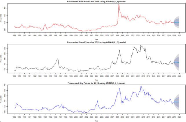
Figure 5. Forecast for year 2019 and original observations of rice prices using ARIMA(5,1,4), corn prices using ARIMA(6,1,3) and soybeans prices using ARIMA(6,1,1). Dark, grey-colored bands indicate 80% forecast confidence, while lighter grey-colored bands indicate 95% confidence.
Figure 5 displays the historical price trends from 1988 to 2018 for rice, corn, and soybeans, along with forecasted monthly values for 2019, extending each series one year ahead using ARIMA(5,1,4), ARIMA(6,1,3) and ARIMA(6,1,1) time series models respectively shown with shaded confidence intervals. The forecast for rice prices shows a slight upward movement or stabilization, suggesting the model expects rice prices to recover marginally, corn prices for 2019 forecast indicates a stable continuation like (2017-2018) period, while the forecast for soybean prices suggests a modest increase or leveling off in 2019, following the downward trend shown from the 2012 peak. The price for rice, corn, and soybeans in 2019 is expected to remain around USD 400, 180, and 360, respectively.
3.3. Model Diagnostics
Based on AIC values and performance on in-sample and out-of-sample data, ARIMA(5,1,4), ARIMA(6,1,3) and ARIMA(6,1,1) were chosen as the best models out of the list of candidate models for forecasting rice, corn, and soybean prices respectively. Testing was conducted on the chosen models to determine if any autocorrelations are present in the residuals, with the null hypothesis: There is no autocorrelation in the series, at a set threshold of 0.05. The results of the Ljung box test of residuals of the three models can be seen in Table 5. The results show that there is no autocorrelation in the rice series; however, autocorrelation is present in corn and soybean prices.
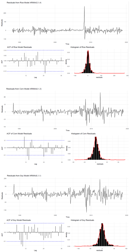
Figure 6. Residual plots of ARIMA(5,1,4), ARIMA(6,1,3) and ARIMA(6,1,1).
Table 5. Ljung-Box test result.

Ljung-Box test

Q* = 14.186, df = 14, p-value = 0.43591

ARIMA(5,1,4)

lags=24

Q* = 39.369, df = 14, p-value =0.00031977

ARIMA(6,1,3)

lags=24

Q* = 39.546, df = 16, p-value = 0.00090666

ARIMA(6,1,1)

lags=24

The p-value for ARIMA(5,1,4) for rice exceeded 0.05. This implies that there is no significant evidence of residual autocorrelation up to lags 24. However, significant evidence of residual autocorrelation was found in ARIMA(6,1,3) for corn and ARIMA(6,1,1) for Soybeans, up to lag 24. Subsequent tests of all candidate models yield similar levels of significance. These consistently significant results in the residuals of the ARIMA(6,1,3) and ARIMA(6,1,1) price models can be solved by using higher-order models.
4. Discussion
In the literature, existing research has mostly examined agricultural prices through regional or national lenses . In contrast, our global approach, utilizing longstanding World Bank data, captures essential cross-border price dynamics that reveal macro-level patterns often hidden in localized studies. This approach and use of World Bank data provide unique advantages. Where others employ complex hybrid methods , we demonstrate that a carefully specified ARIMA model framework can achieve similar predictive accuracy while maintaining crucial interpretability for policymakers. Furthermore, the dataset provides insights into structural market transformations that shorter analyses cannot adequately address. These include trade liberalization effects (WTO price convergence) to climate variability impacts, for example, the 2008 rice price spike linked to Australian droughts and Asian floods.
These methodological choices yield significant practical applications. The large volatility in rice prices (SD = $126.86), consistent with literature findings , highlights its particular susceptibility to climate shocks, export restrictions, and geopolitical instability. This evidence strongly suggests that import-dependent nations should prioritize strategic diversification and buffer stock policies. Similarly, the persistent autocorrelation in our corn and soybean models points to potential unmodeled factors, including biofuel demand shocks and speculative trading patterns, which warrant future investigation. When combined with domain expertise, our modeling framework could enable governments and agribusinesses to (a) better anticipate global price fluctuations, (b) optimize trade decisions, (c) strengthen food security planning, and (d) engage in more sustainable agriculture. Future research directions could productively explore multivariate extensions such as ARIMA with eXogenous variables (ARIMAX) and seasonal ARIMAX (SARIMAX), and machine learning applications to further enhance forecasting precision.
5. Conclusions
Rice, corn, and soybeans hold significant importance globally, as they play a crucial role in ensuring food security. Consequently, their demand remains high. Due to the influence of various factors, the prices of these commodities tend to fluctuate over time. Therefore, the ability to forecast their prices holds considerable economic importance for policyholders, farmers, and decision-makers. In this study, an ARIMA time series modelling approach was employed to establish a framework for determining the order of the ARIMA model for forecasting the prices of corn, soybeans, and rice based on World Bank prices. Analyzing data spanning from 1988 to 2018, the optimal model orders for forecasting prices in 2019 were identified as ARIMA (5,1,4), ARIMA (6,1,3), and ARIMA (6,1,1) for rice, corn, and soybean, respectively. However, residual analysis of the ARIMA (6,1,3) and ARIMA (6,1,1) models for corn and soybean revealed significant autocorrelation of the residuals up to lag 24. This issue could be resolved by disregarding parsimony and incorporating higher-order lags. Given the volatile nature of commodity prices, enhancing accuracy and extending projections for the long term would involve modifying the model. This could be achieved by integrating more recent pricing data and instituting regular price monitoring practices. Additionally, given the fact that fertilizer and fuel costs often impact on the prices of rice, corn, and soybeans a model that incorporates these variables should be able to offer more realistic forecasts. As such, future work can explore the use of the ARIMAX or SARIMAX model (for commodity prices with seasonal fluctuations), which allows for the inclusion of exogenous variables such as fuel and fertilizer costs. Furthermore, considering the disruptive impact of global events like the COVID-19 pandemic, future research can also focus on modelling price behaviors under such shock conditions to improve preparedness and forecast resilience in times of global uncertainty.
Abbreviations

ACF

Autocorrelation Function

AIC

Akaike Information Criterion

ARIMA

Autoregressive Integrated Moving Average

ARIMAX

Autoregressive Integrated Moving Average with Exogenous Variables

MAPE

Mean Absolute Percentage Error

MAE

Mean Absolute Error

PACF

Partial Autocorrelation Function

RSME

Root Mean Squared Error

SARIMAX

Seasonal Autoregressive Integrated Moving Average with Exogenous Variables

WTO

World Trade Organization

Author Contributions
Bunnel Bernard: Conceptualization, Writing - original draft, Data curation, Formal Analysis, Investigation, Methodology, Project administration, Resource, Software, validation
Linda Francois: Conceptualization, Data curation, Formal Analysis, Investigation, Methodology, Project administration, Resources, Software, validation, visualization, Writing - review & editing
Dwayne Shorlon Renville: Conceptualization, Investigation, Methodology, Project administration, Resources, Validation, Writing - review & editing
Funding
This work is not supported by any external funding.
Data Availability Statement
The data that supports the findings of this study can be found at: https://www.worldbank.org/en/research/commodity-markets (Monthly prices)
Conflicts of Interest
The authors declare no conflicts of interest.
References
[1] Y. J. Mgale, Y. Yan, and S. Timothy, “A Comparative Study of ARIMA and Holt-Winters Exponential Smoothing Models for Rice Price Forecasting in Tanzania,” Open Access Libr. J., vol. 08, p. e7381, 2021,
[2] P. Sirisupluxana and I. Nitithanprapas Bunyasiri, “Risk assessment and risk management decisions: a case study of Thai rice farmers,” Bus. Manag. Rev., vol. 9, no. 3, pp. 200-207, 2018, [Online]. Available:
[3] R. Gök and E. Kara, “Impacts Of The Covid-19 Pandemic On The Agricultural Prices: New Insights From Cwt Granger Causality Test,” J. Res. Econ. Polit. Financ., vol. 5, pp. 76-96, 2020,
[4] S. Frimpong, E. N. Gyamfi, Z. Ishaq, S. Kwaku Agyei, D. Agyapong, and A. M. Adam, “Can Global Economic Policy Uncertainty Drive the Interdependence of Agricultural Commodity Prices? Evidence from Partial Wavelet Coherence Analysis,” Complexity, vol. 2021, 2021,
[5] G. Barrows, S. Sexton, and D. Zilberman, “The impact of agricultural biotechnology on supply and land-use,” Environ. Dev. Econ., vol. 755, pp. 676-703, 2014,
[6] A. Adeosun, R. O. Olayeni, M. I. Tabash, and S. Anagreh, Revisiting the Oil and Food Prices Dynamics: A Time Varying Approach, vol. 19, no. 3. Springer International Publishing, 2023.
[7] S. A. David, J. A. T. Machado, L. R. Trevisan, C. M. C. Inácio, and A. M. Lopes, “Dynamics of commodities prices: Integer and fractional models,” Fundam. Informaticae, vol. 151, no. 1-4, pp. 389-408, 2017,
[8] Darekar and A. A. Reddy, “Forecasting of common paddy prices in India,” J. Rice Res., vol. 10, no. 1, pp. 71-75, 2017, Accessed: May 26, 2025. [Online]. Available:
[9] P. V Cenas, “Forecast of Agricultural Crop Price using Time Series and Kalman Filter Method,” Asia Pacific J. Multidiscip. Res., vol. 5, no. 4, pp. 15-21, 2017.
[10] Darekar and A. A. Reddy, “Forecasting wheat prices in India,” Wheat Barley Res., vol. 10, no. 1, pp. 33-39, 2018, [Online]. Available:
[11] Bisht and A. Kumar, “Estimating Volatility in Prices of Pulses in India: An Application of Garch Model,” Econ. Aff. (New Delhi), vol. 64, no. 3, pp. 513-516, 2019,
[12] R. W. Divisekara, G. J. M. S. R. Jayasinghe, and K. W. S. N. Kumari, “Forecasting the red lentils commodity market price using SARIMA models,” SN Bus. Econ., vol. 1, no. 1, pp. 1-13, 2021,
[13] S. Luo, L. Y. Zhou, and Q. F. Wei, “Application of SARIMA model in cucumber price forecast,” Appl. Mech. Mater., vol. 373-375, pp. 1686-1690, 2013,
[14] L. Mao, Y. Huang, X. Zhang, S. Li, and X. Huang, “ARIMA model forecasting analysis of the prices of multiple vegetables under the impact of the COVID-19,” PLoS One, vol. 17, no. 7, p. e0271594, 2022,
[15] H. Adanacioglu and M. Yercan, “An analysis of tomato prices at wholesale level in Turkey: An application of SARIMA model,” Custos e Agronegocio, vol. 8, no. 4, pp. 52-75, 2012.
[16] R. M. Mutwiri, “Forecasting of Tomatoes Wholesale Prices of Nairobi in Kenya: Time Series Analysis Using Sarima Model,” Int. J. Stat. Distrib. Appl., vol. 5, no. 3, pp. 46-53, 2019,
[17] R. C. T. de Souza, O. Guedes Filho, M. A. R. dos Santos, and L. D. S. Coelho, “Monthly Closing Price Forecasting of Soybean Grain in Paraná Using Sarima Modeling With Intervention,” J. Geospatial Model., vol. 2, no. 1, pp. 27-44, 2016,
[18] “Commodity Markets.” Accessed: Jun. 02, 2025. [Online]. Available:
[19] P. C. Padhan, “Application of ARIMA Model for Forecasting Agricultural Productivity in India,” J. Agric. Soc. Sci., vol. 8, no. 2, pp. 50-56, 2012.
[20] S. U. Pepple and E. E. Harrison, “Comparative Performance of Garch and Sarima Techniques in the Modeling of Nigerian Broad Money,” CARD Int. J. Soc. Sci. Confl. Manag., vol. 2, no. 4, pp. 2536-7242, 2017, [Online]. Available:
[21] S. N. Kumari and A. Tan, “Modeling and forecasting volatility series: With reference to gold price,” Thail. Stat., vol. 16, no. 1, pp. 77-93, 2018.
[22] Kathayat and A.. Dixit, “Paddy price forecasting in India using ARIMA mode,” J. Crop Weed, vol. 17, no. 1, pp. 48-55, 2021,
Cite This Article
  • APA Style

    Bernard, B., Francois, L., Renville, D. S. (2025). Forecasting the International Market Prices for Rice, Corn and Soybeans Using ARIMA Time Series Modelling. International Journal of Agricultural Economics, 10(4), 170-182. https://doi.org/10.11648/j.ijae.20251004.13

    Copy | Download

    ACS Style

    Bernard, B.; Francois, L.; Renville, D. S. Forecasting the International Market Prices for Rice, Corn and Soybeans Using ARIMA Time Series Modelling. Int. J. Agric. Econ. 2025, 10(4), 170-182. doi: 10.11648/j.ijae.20251004.13

    Copy | Download

    AMA Style

    Bernard B, Francois L, Renville DS. Forecasting the International Market Prices for Rice, Corn and Soybeans Using ARIMA Time Series Modelling. Int J Agric Econ. 2025;10(4):170-182. doi: 10.11648/j.ijae.20251004.13

    Copy | Download

  • @article{10.11648/j.ijae.20251004.13,
      author = {Bunnel Bernard and Linda Francois and Dwayne Shorlon Renville},
      title = {Forecasting the International Market Prices for Rice, Corn and Soybeans Using ARIMA Time Series Modelling
    },
      journal = {International Journal of Agricultural Economics},
      volume = {10},
      number = {4},
      pages = {170-182},
      doi = {10.11648/j.ijae.20251004.13},
      url = {https://doi.org/10.11648/j.ijae.20251004.13},
      eprint = {https://article.sciencepublishinggroup.com/pdf/10.11648.j.ijae.20251004.13},
      abstract = {Rice, corn, and soybeans are among the most widely cultivated crops, making them crucial for global food security and the economic well-being of many countries. Like many other crops, the global prices for these commodities are prone to fluctuations due to unfavorable weather conditions, natural disasters (like flooding), global demand, and economic crises. Consequently, their prices are subject to significant changes and volatility. Forecasting and modelling these prices offer valuable insights to policymakers and local growers within the agricultural sector. While there is a plethora of studies focusing on forecasting prices based on data obtained for a specific locality, country, or region, there is a paucity of publications that take on a more global outlook for rice, corn, and soybeans. The objective of this study is to use an Autoregressive Integrated Moving Average (ARIMA) process to model and forecast the international market prices of milled rice (5% broken), corn, and soybeans. We relied on World Bank data covering the period from 1988 to 2018 to construct several time series models. The average prices for milled rice, corn, and soybeans are $344.47, $144.48, and $334.72 (USD) per metric ton, respectively. The results of the model selection procedure indicate that the ARIMA (5,1,4), ARIMA (6,1,3), and ARIMA (6,1,1) models best fit the prices of milled rice, corn, and soybeans, respectively. Furthermore, these models offer the best in-sample and out-of-sample performances. The accuracy of the projected values, derived from the chosen models, was evaluated by calculating several metrics, including the mean absolute error (MAE), mean squared error (MSE), root mean square error (RMSE), and mean absolute percentage error (MAPE). This paper highlights the utility and applicability of the ARIMA model as a powerful tool for forecasting agricultural prices. Our modeling framework could enable governments and agribusinesses to (a) better anticipate global price fluctuations, (b) optimize trade decisions, (c) strengthen food security planning, and (d) engage in more sustainable agriculture.},
     year = {2025}
    }
    

    Copy | Download

  • TY  - JOUR
    T1  - Forecasting the International Market Prices for Rice, Corn and Soybeans Using ARIMA Time Series Modelling
    
    AU  - Bunnel Bernard
    AU  - Linda Francois
    AU  - Dwayne Shorlon Renville
    Y1  - 2025/07/07
    PY  - 2025
    N1  - https://doi.org/10.11648/j.ijae.20251004.13
    DO  - 10.11648/j.ijae.20251004.13
    T2  - International Journal of Agricultural Economics
    JF  - International Journal of Agricultural Economics
    JO  - International Journal of Agricultural Economics
    SP  - 170
    EP  - 182
    PB  - Science Publishing Group
    SN  - 2575-3843
    UR  - https://doi.org/10.11648/j.ijae.20251004.13
    AB  - Rice, corn, and soybeans are among the most widely cultivated crops, making them crucial for global food security and the economic well-being of many countries. Like many other crops, the global prices for these commodities are prone to fluctuations due to unfavorable weather conditions, natural disasters (like flooding), global demand, and economic crises. Consequently, their prices are subject to significant changes and volatility. Forecasting and modelling these prices offer valuable insights to policymakers and local growers within the agricultural sector. While there is a plethora of studies focusing on forecasting prices based on data obtained for a specific locality, country, or region, there is a paucity of publications that take on a more global outlook for rice, corn, and soybeans. The objective of this study is to use an Autoregressive Integrated Moving Average (ARIMA) process to model and forecast the international market prices of milled rice (5% broken), corn, and soybeans. We relied on World Bank data covering the period from 1988 to 2018 to construct several time series models. The average prices for milled rice, corn, and soybeans are $344.47, $144.48, and $334.72 (USD) per metric ton, respectively. The results of the model selection procedure indicate that the ARIMA (5,1,4), ARIMA (6,1,3), and ARIMA (6,1,1) models best fit the prices of milled rice, corn, and soybeans, respectively. Furthermore, these models offer the best in-sample and out-of-sample performances. The accuracy of the projected values, derived from the chosen models, was evaluated by calculating several metrics, including the mean absolute error (MAE), mean squared error (MSE), root mean square error (RMSE), and mean absolute percentage error (MAPE). This paper highlights the utility and applicability of the ARIMA model as a powerful tool for forecasting agricultural prices. Our modeling framework could enable governments and agribusinesses to (a) better anticipate global price fluctuations, (b) optimize trade decisions, (c) strengthen food security planning, and (d) engage in more sustainable agriculture.
    VL  - 10
    IS  - 4
    ER  - 

    Copy | Download

Author Information
  • Department of Mathematics, Physics and Statistics, University of Guyana, Georgetown, Guyana

    Biography: Bunnel Bernard is a lecturer at the University of Guyana. He holds a BSc in Mathematics from the University of Guyana (2015) and an MSc in Applied Modelling and Quantitative Methods from Trent University (2024). His master’s research focused on developing a mathematical model and modelling structure for agricultural planning. Currently, his research interests lie in weather simulation and modelling, evapotranspiration estimation and modelling, multi-objective optimization, AquaCrop yield estimation, and the development of agricultural planning models. He is passionate about using applied mathematics and quantitative methods to address real-world challenges in agriculture and environmental systems. Through his work, he aims to contribute to more informed decision-making in climate-resilient agriculture and resource management by integrating modelling, data, and optimization strategies.

    Research Fields: weather simulation and modelling, Reference Evapotranspiration estimation and modelling, Multi-objective optimization, AquaCrop yield estimation, and Agricultural planning models.

  • Department of Mathematics, Physics and Statistics, University of Guyana, Georgetown, Guyana

    Biography: Linda Francois is a Lecturer at the University of Guyana, Department of Mathematics, Physics, and Statistics. She holds an MSc in Ac-tuarial Science with a minor in Finance from the University of Nebraska-Lincoln and a BSc in Statistics from the University of Guyana. Her work integrates statistical and mathematical analysis with applied research in public health, urban flood resilience, and time series modelling. She has contributed to studies on inclusive urban flood resilience and public health challenges in the Demerara-Mahaica region. Linda is committed to academic excellence, student development, and interdisciplinary collaboration supporting data-driven policy and sustainable development in Guyana.

    Research Fields: Applied Statistical Modelling, Public Health Statistics, Urban resilience and Environmental Statistics, Development Studies, Biostatistics.

  • Department of Mathematics, Physics and Statistics, University of Guyana, Georgetown, Guyana

    Biography: Dwayne Shorlon Renville is a lecturer in the Department of Mathematics, Physics, and Statistics at the University of Guyana. He obtained his Bachelor’s and Master’s degrees in Mathematics from the University of Guyana, Guyana, and the University of the West Indies, Mona Campus, Jamaica, respectively. He recently completed his doctoral degree in Innovation in Global Development at Arizona State University, USA, where his research focus has since been on inclusive development, urban flood resilience, and their fusion, inclusive urban flood resilience. As a freshly minted scholar of innovation in global development, Dr. Renville is spearheading a number of research papers in these fields. Relying on his mathematics background, Dr. Renville is engaged in other research projects and collaborations in other fields such as public health and biostatistics.

    Research Fields: Development Studies, Inclusive Development, Flood Resilience, Biostatistics, Urban Studies.