Abstract
Exchange rate movement is perceived as a very important factor in influencing the performance of the agriculture sector. When the currency of the exporting country depreciates against the trading partners’ currencies tends to stimulate demand and improve export earnings. An increase in value of the currency against the other trading partners’ currencies (e.g. USD) tend to affect the costs of production that may affect aggregate agricultural supply. However, the linkage of the exchange rate and agricultural export growth in particular traditional exports such as coffee has never been properly and intensively documented for appropriate decision-making in Tanzania. Therefore, this study was set to assess how exchange rate variability has affected coffee export growth in Tanzania. The study made use of time series data from 1991 to 2022 using the vector error collection model (VECM). Given the influences other than the real effective exchange rate on the export of coffee growth, we discriminately incorporated inflation rate, discount rate, and money supply, as the independent variables. Yearly data (1991-2022) obtained from the Bank of Tanzania and the International Coffee Organization were used for the analysis. The results from this study reveal that the real effective exchange rate has an enormous positive impact on coffee export growth in the long run. This implies that, the depreciation of the domestic currency against USD has advantage on coffee export growth when considering the demand side as it tends to stimulate coffee demand in the rest of the world, thus leading to an increase in export volume and revenue which helps to foster coffee export growth. However, in the supply side, this depreciation should be carefully monitored as excess depreciation may end up by rising inputs prices especially those inputs imported such as fertilizers, agrochemical, aggrotech and agro machineries that may intern affect the production level. The study ends by concluding, that it is imperative for the Central Bank to carefully observer exchange rate fluctuations and implement appropriate monetary policy strategies in favour of the agriculture sector in particular exportable crops such as coffee. This will help to manage the risks and opportunities that may arise in coffee export growth associated with currency movement.
Keywords
Coffee Export Growth, Real Effective Exchange Rate, Inflation Rate, Discount Rate, Money Supply Growth Rate
1. Background of the Study
Instability in macroeconomic variables such as exchange rate, imposes uncertainties and increases the real cost on farmers' decision-making, reduces farms' profitability, and impairs agricultural performance in terms of production as well as marketing.
Exchange rate transmission channels exhibit a significant effect on farm export performance. When the currency of the exporting country depreciates against the trading partners’ currencies tend stimulate demand for exports and consequently improve export earnings. In this case, the way exchange rates vary tends to affect agricultural output and aggregate demand in the exporting and importing countries respectively
| [1] | Athanasius, N. (2017). An analysis of banks’ credit and agricultural output in Nigeria: 1980-2014. International Journal of Innovative Finance and Economic Research 5(1), 54, 66. |
| [7] | George, W. (2022). Export performance of the horticultural sub-sector in Tanzania. In Trade and Investment in East Africa (pp. 293-313). Springer, Singapore. |
| [11] | Iliyasu, A. S. (2019). An empirical analysis of the impact of interest rates on agriculture is the exchange rate is the culprit. Federal Reserve Bank of St. Louis Review, Journal of Social Sciences, 5(1), 613. |
| [12] | Kargbo, J. M. (2006). Exchange rate volatility and agricultural trade under policy reform in South Africa. Development Southern Africa, 23(01), 147-170. |
[1, 7, 11, 12]
. Either excessive increase or decrease in the value of the currency against the other trading partners’ currencies tends to decrease/increase the costs of production in terms of farm input prices and consequently affect the aggregate agricultural supply.
In Tanzania, since the economic liberalization started, in particular from 1993/94 all export restrictions were eliminated and the economy started to exhibit growth in which agricultural export earnings contributed significantly. This was realized as a result of the major policy reforms that the government implemented to achieve a positive trade balance and increase agricultural exportable products competitiveness in the international markets. In these reforms, the Government abolished the export licensing systems for traditional crops, eliminated the requirement of registration of exporting companies and dropped the foreign exchange surrender requirement
| [15] | Marwa, N. (2019). Unlocking Coffee Production in Tanzania: What Does the Future Holds. Policy Brief, (7). |
[15]
. The ultimate goal of the reform program was to increase the profitability of cash crops by introducing multiple channels for marketing them and allowing farmers to receive a high share of the proceeds from export sales.
The relaxation of the trade restrictions was also to correct the exchange rate misalignment reflected in a sharp depreciation of the real effective exchange rate. Those government initiatives including the adoption of a floating exchange rate policy, helped to enhance farm export growth performance in particular traditional exports such as coffee. However, regardless of the critical contribution the coffee sector has to the national economy including being among the major sources of foreign exchange earnings, its growth in terms of export value has been low exhibiting up and down trends with its share of total national export earnings declining for some periods (
Table 1).
Table 1. Coffee Export Performance (1995-2022).
| Total exports (goods and services) | Volume '000' Tonnes | Coffee, value (Mill. of USD) | Unit Price USD/Tonne | Coffee value share |
1995 | 680.9 | 43.5 | 60.3 | 1386.7 | 8.9 |
2000 | 667.6 | 46.7 | 80.2 | 1750.5 | 12.0 |
2005 | 1242.5 | 43.1 | 53.3 | 1226.5 | 4.3 |
2010 | 2699.8 | 42.7 | 94.3 | 2230.8 | 3.5 |
2015 | 4621.9 | 51.8 | 158.3 | 3093.4 | 3.4 |
2020 | 4699.8 | 59.4 | 145.1 | 2468.4 | 3.1 |
Source: Computed using data from BOT and ICO, 2020
This gives rise to an important question of whether the observed export growth volatility is partly associated with the movement of the exchange rate instability. Given the importance of coffee in the export sector, of which more than 90 percent of total national coffee produced which is equivalent to about 64,000 tonnes are exported, it is worth exploring whether the exchange rate instability might have affected its export growth in any way.
Therefore, this study was set to assess the effects of exchange rate variability on coffee export growth in Tanzania. To this end, the contribution of this study is in two ways as follows: - First, this helps to fill the vacuum of information on the exchange rate dynamics and the way it affects coffee export growth in Tanzania by closing the gap between theory and practice. Second, the finding of the study also helps to inform policymakers and farmers on understanding how monetary policy through the exchange rate transmission channel feeds into farm operations. More importantly the results from this study will help to enhance the efficient coffee value chain that enables high crop productivity and quality to compete in the global markets for enhancing export earnings growth.
1.1. A Brief Overview of the Coffee Sector
Coffee has been among the major cash crops having a large contribution to the economy of Tanzania. It is also among the important traditional cash crops with a long history since started to be grown as a source of foreign exchange earnings. The national production per annum is estimated to range to an average of 55,920.0 MT, of which 70 percent of the total national production is Arabica, and 30 percent is Robusta
| [15] | Marwa, N. (2019). Unlocking Coffee Production in Tanzania: What Does the Future Holds. Policy Brief, (7). |
[15]
. The crop is grown mostly by small farmers mainly for commercial purposes, commanding 90 percent of the total national output, while the remaining (10 percent) comes from the estates
| [20] | Samoei, S. K., & Kipchoge, E. K. (2021). Drivers of Horticultural Exports in Kenya. Journal of Economics and Financial Analysis, 4(2), 27-44. |
[20]
.
The average national productivity is 1kg per tree of clean coffee which is quite below the potential production of 3 kg/tree per crop season
| [15] | Marwa, N. (2019). Unlocking Coffee Production in Tanzania: What Does the Future Holds. Policy Brief, (7). |
[15]
. This productivity level is regarded as among the lowest productivity in the world
| [6] | FAO (2020); Production Quantity Data. |
[6]
.
More than 90% of the total national coffee produced per annum is exported, contributing 1 percent of world coffee output
. It is estimated that about 2.5 percent of the total national exports of goods and services (equivalent to 6,061.3 million. USD) in 2022 was obtained from the coffee exported. Therefore, enhancing the performance of the coffee sector would have a great advantage not only for producers but also for the national economy at large.
1.2. The Relationship Between Exchange Rate and Coffee Export Growth
Overall, exchange rate movement effects on coffee export growth are complex. The magnitude and direction of these effects depend on specific economic conditions, the stability of exchange rate movements, and the responsiveness of both coffee producers and consumers to these changes. Coffee is one of Tanzania's most traded commodities in the global markets and the export revenue is sensitive to fluctuations in exchange rates.
There are several reasons why the exchange rate variability has been considered as a key factor for coffee export growth. First, coffee export contracts in Tanzania are priced and paid in foreign currency (usually USD). Therefore, exchange rate variability may affect coffee export earnings valued in domestic currency. Second, export contracts involve long time lags in the date for coffee sales and settlement of payments which may increase the extent of uncertainty.
Thirdly, most of the farm inputs used in coffee production including fertilizers, pesticides, and machinery are imported; this importation is made by foreign currency and it seems to have much impact on the costs of production.
Therefore, it is essential to recognize that the relationship between coffee export growth and the exchange rate is complex and can be influenced by multiple factors, including those specific to Tanzania's domestic economic policies and the global coffee market. As such police makers and coffee industry stakeholders need to consider a comprehensive approach to foster sustainable growth in the coffee export sector.
2. Literature Review
2.1. Theoretical Review
The theoretical literature offers many models explaining the association between monetary policy through its channels which affect the real economy. Among the monetary policy transmission channels that are mostly considered to affect agricultural exports growth is the exchange rate transmission channel. The monetary approach to exchange rate theory seeks to explain exchange rate movements primarily through the influence of monetary factors specifically money supply and demand. This approach emphasizes the role of the Central Bank and monetary policy in determining exchange rates
| [12] | Kargbo, J. M. (2006). Exchange rate volatility and agricultural trade under policy reform in South Africa. Development Southern Africa, 23(01), 147-170. |
[12]
.
This study, therefore, is built into the exchange rate determination of the monetary theory which explains the concept of the exchange rate as the monetary policy channel to provide the theoretical linkages between the monetary policy transmission channel and agricultural output and export growth with a view about how it can affect farm sector performance. The theory of monetary approach hypothesizes that, any attempt by the monetary authority to change the money supply while keeping the money supply constant in the rest of the world will decrease the exporting country's exchange value. Linking this to the farm sector, Devadoss
| [4] | Devadoss, S. (1985). The impacts of monetary policies on US agriculture (United States). |
[4]
suggested that, as the monetary policy intends to stimulate economic growth then, has to increase the money supply; this, in turn, will decrease the value of the currency and ultimately lead to higher export demand for farm products by the rest of the world
| [3] | Chambers, R. G., & Just, R. E. (1982). An investigation of the effect of monetary factors on China’s food industry. |
| [22] | Shane, M., Roe, T., & Somwaru, A. (2008). Exchange rates, foreign income, and US |
[3, 22]
.
In the environment of the economy practicing an expansionary monetary policy stance tends to affect the exchange rate of the domestic currency/devalue the domestic currency against the trading partner's currency. The decrease in the value of the domestic currency creates demand pressure on the domestic goods in the global markets and thus increases net export as explained in the below equation 1: -
 (1)
(1)Where by; M = money supply; Ir = lending rates by commercial banks; Cr = Credit; E = Exchange rates, NX = net export; and Y represents output.
This transmission mechanism is becoming a standard feature in the macroeconomics and money and banking environment.
Therefore, the exchange rate factor pulls a foreign country to import goods from another country and thus, influences farmers' decisions to increase production output. This implies that as an exporting currency is relatively low in value against the other foreign currencies, it will effectively make her commodities less expensive in the foreign markets.
Thus, currency depreciation is expected to make domestic agricultural exports relatively cheaper and encourage exports, gaining competitiveness in foreign markets
| [5] | Dushmanitch, V. Y., and Darroch, M. A. G. (1990). An economic analysis of the impacts of monetary policy on South African agriculture. |
| [14] | Mao, R. (2019). Exchange rate effects on agricultural exports: A firm-level investigation of China’s food industry |
| [22] | Shane, M., Roe, T., & Somwaru, A. (2008). Exchange rates, foreign income, and US |
[5, 14, 22]
.
2.2. Empirical Literature Review
Several empirical studies have investigated the effect of exchange rate movement on farm output, farm prices, farm income, and farm exports in the short run and the long run. Among this plethora of research endeavors, some found a positive significant relationship while others reported the opposite. Another study indicated that the effect of exchange rate variability is ambiguous.
Udeaja & and Elijah
| [25] | Udeaja, E. A., & Elijah, U. A. (2014). Effect of monetary policy on the agricultural sector in Nigeria. |
[25]
conducted a study to examine the effect of monetary policy on the agricultural sector in Nigeria by utilizing time-series data from 1970 to 2010. The study adopted an Auto-Regressive Distributed Lag (ARDL) Bound Test approach by capturing both monetary and non-monetary policy variables such as lending rate, commercial bank credit to the agriculture sector, exchange rate, government expenditure, and inflation rate. The results showed that among the explanatory variables used in the study, the exchange rate had a positive and statistically significant effect on agriculture output in Nigeria.
In the study by Athanasius
| [1] | Athanasius, N. (2017). An analysis of banks’ credit and agricultural output in Nigeria: 1980-2014. International Journal of Innovative Finance and Economic Research 5(1), 54, 66. |
[1]
the relationship between banks' credit and agricultural sector performance in Nigeria from 1980 to 2014 was investigated using LSM and VECM. The study found an exchange rate to have a positive and statistically significant relationship with agricultural Gross Domestic Product (GDP).
Using the Vector Error Correlation Model (VECM), Kargbo
| [12] | Kargbo, J. M. (2006). Exchange rate volatility and agricultural trade under policy reform in South Africa. Development Southern Africa, 23(01), 147-170. |
[12]
investigated the supply and demand relationships for agricultural trade flows in South Africa. The findings from the study observed that mainly exchange rate volatility harmed the country's farming business.
Mao
| [14] | Mao, R. (2019). Exchange rate effects on agricultural exports: A firm-level investigation of China’s food industry |
[14]
investigated the relationship between real exchange rates and agricultural exports in China; employing Panel Regression Model. The study revealed that real appreciation reduces export quantities and the probability of entering the destination market.
Samoei & Kipchoge
| [20] | Samoei, S. K., & Kipchoge, E. K. (2021). Drivers of Horticultural Exports in Kenya. Journal of Economics and Financial Analysis, 4(2), 27-44. |
[20]
examined major drivers behind horticultural exports in Kenya for the period 2005 to 2017 using the co-integration method. The study results explore that; the exchange rate had a positive impact on horticulture exports in Kenya.
Elius et al.,
| [2] | Elias, A., Dachito, A., & Abdulbari, S. (2023). The effects of currency devaluation on Ethiopia’s major export commodities: The case of coffee and khat: Evidence from the vector error correction model and the Johansen co-integration test. Cogent Economics & Finance, 11(1), 2184447. |
[2]
conducted a study to establish the effect of currency devaluation on major export commodities in Ethiopia using the Vector Error Collection Model and the Johansen co-integration. The study revealed that devaluation of the real effective exchange rate had a positive and significant relationship with the value of major export commodities in the long run meaning that a decrease in the value of domestic currency promotes exports in the long run.
Mehare & and Edriss
| [16] | Mehare, A., & Edriss, A. K. (2013). Evaluation of the Effect of Exchange Rate Variability on the Export of Ethiopia’s Agricultural Product: A Case of Coffee. Margin: The Journal of Applied Economic Research, 7(2), 171–183. https://doi.org/10.1177/0973801013483506 |
[16]
, studied the effect of exchange rate variability export of coffee in Ethiopia. The study employed an Auto-Regressive Distributed lag (ARDL) Bound Test approach. The results indicate that, exchange rate variability hurt the export of coffee in the short run, but was insignificant in the long run implying that, the exchange rate over time has been favoring the export performance of coffee in Ethiopia.
Shane & Samwaru
| [22] | Shane, M., Roe, T., & Somwaru, A. (2008). Exchange rates, foreign income, and US |
[22]
conducted a study to investigate the effect of exchange rate on agricultural export using Directed Acyclic Graph (DAG) technique. The study was to identify the inverted fork causal relationship of exchange appreciation and agricultural exports. The study found, that a one percent appreciation of the dollar relative to trade partners' trade-weighted currencies decreases total agricultural exports by about 0.5 percent.
Montenegro & Miranda [19], investigated the relationship pattern between agricultural exports as an independent variable and exchange and interest rates as independent variables for the Mexican economy using multiple regression analysis and the Granger causality test. The result was different from the aforementioned studies. From the findings, it was revealed that agricultural exports in Mexico have not been affected by variations in the exchange rate or by a monetary policy of Mexico in the period 1993 to 2017.
George
| [7] | George, W. (2022). Export performance of the horticultural sub-sector in Tanzania. In Trade and Investment in East Africa (pp. 293-313). Springer, Singapore. |
[7]
, conducted a study on export performance of the horticultural sub-sector in Tanzania using the Co-integration technique to examine a long-run relationship among the time series data of monetary variables. The study revealed that the real exchange rate influenced horticultural export performance in the long run.
Hong
| [9] | Hong, T. T. K. (2016). Effects of exchange rate and world prices on the export price of Vietnamese coffee. International Journal of Economics and Financial Issues, 6(4), 1756-1759. |
[9]
, studied the effect of exchange rate and world prices on the export prices of Vietnamese Coffee by applying time series data of 34 years. The exchange rate was found to affect coffee price fluctuation which ultimately influences the export growth performance.
Tumaini
| [24] | Tumaini, H. D. (2018). Influence of Exchange Rate Volatility on coffee exports in Tanzania from 1996 to 2016 (Doctoral dissertation, The Open University of Tanzania). |
[24]
, examined the volatility of the real exchange rate of the currency of Tanzania and its influence on coffee exports. Time series data spanning from 1996-2016 was analyzed using a gravity model to examine the existing relationship between the dependent and independent variables. The results revealed that, in the long run, variation in coffee exports can be explained only by the real exchange rate.
Rutashoborwa
| [19] | Rutashoborwa, P. M. H. (2013). Impact of International Trade on Coffee Industry: The Case of Kagera Region in North-West Tanzania |
[19]
, in his doctoral dissertation also utilized the Least Square Method and time series analysis in the form of a linear equation to examine the impact of international trade on the coffee export industry in Tanzania. The results obtained revealed that the exchange rate had implications on running production costs in the coffee industry as required inputs are imported at a high price and therefore affect coffee production.
Mlay
| [17] | Mlay, N. (2020). Assessing the Effect of Agricultural Export Values on Foreign Exchange Rate in Tanzania |
[17]
, used Vector Auto-regression and the Granger causality test to assess if there is a long-run relationship between agricultural export values and foreign exchange rates utilizing data from 1990 to 2019. The study found that there is a causality between total agricultural exports and the foreign exchange rate in Tanzania whereby the foreign exchange rate causes agricultural exports and not otherwise. It also revealed that, there is a long-run relationship that exists between agricultural exports value and foreign exchange rate in Tanzania.
Moh’d
| [18] | Moh’d, A. V. (2020). The effect of exchange rate, inflation rate, interest rate and economic growth on agriculture export earnings in Tanzania |
[18]
, employed Multiple regression analysis to examine the effects of selected macroeconomic variables such as exchange rate, inflation rate, interest rate, and economic growth on agricultural export earnings in Tanzania covering the period 1990 to 2019. The study findings showed insignificant relationship between exchange rate and agricultural export earnings. However, the inflation rate and interest rate found to have positive and significant influence on agricultural export earnings in Tanzania.
Generally, from the reviewed literature, variability in the exchange rate has been referenced to affect farm export performance in different environments and magnitudes. However, the direction of the influence of exchange rate on agricultural export performance from the reviewed literature is not uniform. For instance, Moh’d
| [18] | Moh’d, A. V. (2020). The effect of exchange rate, inflation rate, interest rate and economic growth on agriculture export earnings in Tanzania |
[18]
found exchange rates to have an insignificant influence on agricultural exports earnings unlike Mlay
| [17] | Mlay, N. (2020). Assessing the Effect of Agricultural Export Values on Foreign Exchange Rate in Tanzania |
[17]
and Tumaini
| [24] | Tumaini, H. D. (2018). Influence of Exchange Rate Volatility on coffee exports in Tanzania from 1996 to 2016 (Doctoral dissertation, The Open University of Tanzania). |
[24]
who found exchange rate to have positive and significant influence on agricultural export earnings in the long-run in Tanzania. Moreover, there is insufficient evidence from studies particularly focussing on the effect of exchange rate variability on specific traditional exports such as coffee in Tanzania. Therefore, to answer the ambiguity that surrounds the effects of exchange rate variability on coffee export growth, there is a need for further studies to focus on coffee export growth in Tanzania with continuous and exchange rate variability.
3. Methodology of the Study
The study used secondary annual time series data for all the variables under consideration with 31 observations between 1991 and 2022. Variables under this study are Coffee export growth (CEG), real Effective Exchange Rate (REER), Discount rate (DISCR), Inflation (INF) and Money Supply Annual Growth Rate (M2).
The data were obtained from the Bank of Tanzania (BOT) various reports and publications; Tanzania Coffee Board (TCB) and the International Coffee Organization (ICO) various reports. The study performed both descriptive analysis as well regression analysis to characterize and gauge the relationship between coffee export growth, exchange rate, and other relevant macroeconomic variables. to discuss and analyze different issues regarding the study objective. In the analysis, descriptive statistics in the form of tables and graphs were used. In the econometric method of analysis part, the researcher employed the Johansen Co-Integration and Vector Error Correlation (VECM) model to tests the existing relationship between dependent and independent variables under the study. A diagnostic test was also performed to check the fitness of the model applied. The tool used in the data analysis is Eviews version 13.
3.1. Variables Selection and Their Measurements
The variables under this study have been explained in detail together with how to measure them and their relationship (between dependent and independent variables). The researcher considered four macroeconomic variables which are real effective exchange rate, inflation rate, discount rate and annual growth money supply. These variables were selected and examined to see how they influence on coffee export growth because they have a critical role through monetary policy transmission channels and play a meaningful role in the determination of agricultural export growth in most of the less developed countries such as Tanzania. These variables were selected because they have a huge impact on the economy development especially for those countries depending on agriculture like Tanzania.
Table 2. Summary of Variables.
Variable | Measurement | Expected relationship |
CEG | Measured as annual coffee exports valued in millions of USD | |
REER | Real effective exchange rate | + |
INF | Headline inflation is a change in the price level of the entire CPI basket. | - |
DISCR | The discount rate refers to a rate at which commercial banks borrow funds from the central bank expressed in terms of percent | - |
M2 | The money supply growth rate refers to the percent of the total amount of money circulating within an economy | + |
Source: Researcher (2023)
Table 2 above summarises expected relationship between the dependent variable and independent variables
3.2. Empirical Model and Estimation Technique
Empirical Model
The study used the Vector Error Correction (VECM) Model to assess the effect of real effective exchange rate variability on coffee export growth in Tanzania. The variables included in the model are coffee export growth (CEG) as a dependent variable, while real effective exchange rate (REER), discount rate (DISCR), inflation (INF) and broad money supply annual growth rate (M2), were used as explanatory variables. Mathematically, the model was given in the following function form on equation
2: -
CEG= f (REER,DISCR,INF,M2),(2)
The model further was statistically specified as follows: -
CEGt= βo+ β1REERt+ β2DISCRt+ β3INFt+ β4M2t+ µt(3)
Whereby: -
CEG; is the dependent variable representing the total annual value of coffee exported; while REER, DISCR, INF, and M2 are independent variables for real effective exchange rate, discount rate, inflation and broad money supply annual growth rate, respectively.
βo represents a regression constant; β1, β2, β3, and β4 are parameters or estimation coefficients of explanatory variables; and stochastic error terms = µt
In measuring the variables, log transformation has been applied, and hence the natural logarithm forms have been taken for each variable. Through such transformation, the model efficiency is maximized and different measures for each variable are applied, then by natural logarithm the common unit is given for all variables.
Because the data employed were time series needed to capture a long-run and short-run effects on the model, equation 4 was modified by using natural logarithm (ln) as a maximizing function in the analysis. Therefore, the regression equation can be expressed in the mathematical form in a log-linear model as follows: -
LnCEGt=βo+ β1LnREERt+ β2Ln DISCRt+ β3LnINFt+ β4LnM2t+ µt(4)
3.3. Estimation Procedure
The descriptive are in the form of graphs, tables, and percentages. In analyzing the effects of the selected variables on coffee export growth, this study employed co-integration test, stationarity test (unit root test), and Vector Error Correction Model (VECM) estimation. The selection of VECM was in consideration of the time series data behavior analyzed.
Granger & Newbold (1974), have demonstrated that, if time series variables are non-stationary, all regression results with these time series will differ from the conventional theory of regression with stationary series. To get over this problem, data used in this study was analyzed with due consideration of the properties of time series. Therefore, the study tested for the stationarity of the time series data for the variables of interest using the Augmented Dickey-Fuller tests (ADF) as explained in the bellow equation below.
 (5)
(5)Variables which was non-stationary at a level were again checked to ensure the stationary after taking the first difference and second difference.
Before going to further analysis, choosing the optimal lag length is needed. To determine the optimal lag length, different information criteria have been employed including the Akaike Information Criteria (AIC), Schwarz's Bayesian information (SIC), and the Hanna-Quinn Information Criteria(HQC). Practically, the optimal lag length, which is selected by most of these criteria is going to be used. The objective of the information criteria is to select the number of parameters that minimize the value of the information criteria.
After identifying the behavior of the variables used in the study, such as testing for stationarity, a co-integration analysis was important to be conducted. Performing this step was to understand the pattern of the variables and examine at which level they integrate and therefore possible to analyze the long-run relationship between dependent and independent variables. With the nature of the data and the nature of the variables applied Johansen's co-integration test was chosen to test at which level the variables are integrating. Thus, the maximum eigenvalue and trace statistics were generated to determine the number of co-integration vectors in the model.
After performing the co-integration test, it was understood that variables under the study are co-integrated in the long run. We utilized the co-integrating vector to construct the vector error correction model (VECM). The long-run results relationship was obtained after running the error correction term (ECTt-1) which represents a co-integration equation and long-run model.
The equation for the ECT term is given below: -
ECTt-1= (Yt-1-njXt-1–ξmRt-1)(6)
From the model, Yt-1 is the variable of interest (representing the CEG in this model);
Xt-1 and ξm Rt-1 are the order of indigenous variables.
Vector Error Correlation Model, (VECM) is employed to test for the short-run effects of the dependent variables on the dependent variable as specified in the bellow equation: -
 (7)
(7)Where ECT = (ΔCEG t-1 – ØXt); Note that, λ= speed of adjustment with a negative sign,
Ø =

is the long-run parameter;
β1, β2, β3, β4, and β
5 are the coefficients representing short-run dynamics of the model's adjustment in the long run.
A diagnostics check was performed for some fundamental aspects of the model to see how seriously our results could be taken. in terms of the VEC Residual Serial Correlation LM test, Tests for normality and Heteroscedasticity Test, and multicollinearity test.
4. Presentation and Discussion of Findings
4.1. Descriptive Statistics
Before performing econometric estimation, statistical characteristics used in this study were examined to check the behavior of the data used.
Table 3. presents the summary statistics of all variables employed in the study. A descriptive statistic is presented explaining the real coffee export value in real terms and other explanatory variables to give important information to the researcher. The mean, maximum, minimum, and standard deviation values are applied to vigorously check the results. The variable normality level is ascertained from the values of skewness, kurtosis, and Jarque-Bera probability. The results show that the coffee export value varies from 35.22 (Mill. USD) minimum to 186.61 (Mill USD) maximum. From the descriptive results, the REER average value ranges from 95.37 minimum to 115.25 maximum. The standard deviation values reveal that the
CEG and
REER with value 40.21 and 5.48 respectively, deviates further from the mean. The Skewness of the variables shows that coffee export growth has a negative skewness while real effective exchange rates exhibit a positive skewness.
Table 3. Descriptive Statistics Results.
| CEG | REER | DISCR | INF | M2 |
Mean | 111.86 | 104.71 | 14.33 | 10.23 | 17.28 |
Median | 111.19 | 103.95 | 15.99 | 6.13 | 15.09 |
Maximum | 186.61 | 115.25 | 27.00 | 35.28 | 39.26 |
Minimum | 35.22 | 95.37 | 3.70 | 3.29 | 3.76 |
Std. Dev. | 40.21 | 5.48 | 6.65 | 8.08 | 8.09 |
Skewness | -0.11 | 0.27 | 0.31 | 1.54 | 0.76 |
Kurtosis | 2.04 | 2.46 | 2.24 | 4.59 | 3.26 |
Jarque-Bera | 1.25 | 0.74 | 1.24 | 15.46 | 3.08 |
Probability | 0.54 | 0.69 | 0.54 | 0.00 | 0.21 |
Sum | 3467.67 | 3246.06 | 444.31 | 317.16 | 535.54 |
Sum Sq. Dev. | 48508.38 | 899.49 | 1326.82 | 1958.48 | 1962.94 |
Observations | 31 | 31 | 31 | 31 | 31 |
Source: Author’s computations and Eviews 13 output
4.2. Augmented Dickey-Fuller (ADF) Unit Root Test
To avoid spurious and "nonsensical" regression the study undertakes a stationarity test using the Augmented Dickey-Fuller (ADF) test. The ADF test for stationarity shows that all five variables are non-station at the level data as well as a log transformation. The data became stationary after first difference. The results are given in (
Table 4) below: -
Table 4. ADF Stationarity Test Results.
Variable | ADF Calculated value | McKinnon 5% Critical value | Prob. | Order of Integration |
At level | At 1st difference |
LnCEG | -1.5545 | -6.2705** | -2.9639 | 0.0000 | 1(1) |
LnREER | -1.3763 | -4.7650** | -2.9639 | 0.0006 | 1(1) |
LnDISCR | -1.9302 | -5.9476** | -2.9639 | 0.0001 | 1(1) |
LnINF | -1.7995 | -5.6574** | -2.9640 | 0.0001 | 1(1) |
LnM2 | -2.0334 | -10.3894** | -2.9639 | 0.0000 | 1(1) |
**Significant at 5% | | | | |
Source: Authors’ Computation and Eviews 13 Output
4.3. Optimum Lag Selection
The optimal lag length was more imperative in the estimation procedure. To determine the optimal lag length, the information criteria considered were the Akaike Information Criteria (AIC), Schwarz's Bayesian information (SIC), and the Hanna-Quinn Information Criteria(HQC) as indicated in (
Table 5) bellow. The objective of the information criteria is to select the number of parameters that minimize the value of the information criteria.
Table 5 shows the optimum lag structure. The outcome indicates that all of the selection criteria select the optimum lag length of 1 at a 5% level of significance. Hence, the lag length of 1 will be used in estimating the Johansen co-integration test and VECM.
Table 5. Determination of Optimum Lag.
Lag | LogL | LR | FPE | AIC | SC | HQ |
0 | -162.7174 | NA | 0.0002 | 11.3145 | 11.6414 | 11.4191 |
1 | -79.1422 | 122.5771* | 2.12e-05* | 9.009477* | 11.62505* | 9.8462* |
2 | -43.5860 | 35.5562 | 0.0001 | 9.9057 | 14.8099 | 11.4746 |
Source: Authors’ Computation and EViews 13. Output.
4.4. Co-Integration Test (Johansen Co-Integration Test)
After running the unit root test and bound test, the next step was to test for co-integration by using the Johansen co-integration test to ascertain if there is a long-term relationship among these variables. The trace test in (
Table 6 & and
Table 7) showed that the hypotheses of no integration among the variables can be rejected and at least two co-integrating equations at 5% exist. The maximum eigenvalue test confirmed the presence of a long-run relationship among the variables of interest with at least two co-integrating equations at 5%. Because there is co-integration among variables, it indicates that a long-run relationship exists. This means that, even if there is a shock in the short run, which may affect movement in the individual series, they would converge with time (in the long run).
In this regard, both short-run and long-run models shall be estimated, hence the use of the vector error correction model is appropriate.
Table 6. a.Johansen Co-Integration Trace Test.
Hypothesized | | Trace | 0.05 | Prob.** |
No. of CE(s) | Eigenvalue | Statistic | Critical Value | Critical Value |
None * | 0.9631 | 187.6987 | 125.6154 | 0.0000 |
At most 1 * | 0.8356 | 101.8928 | 95.7537 | 0.0177 |
At most 2 | 0.5569 | 54.9493 | 69.8189 | 0.4211 |
At most 3 | 0.4760 | 33.7858 | 47.8561 | 0.5136 |
At most 4 | 0.3590 | 16.9824 | 29.7971 | 0.6414 |
Source: Authors’ Computation and EViews 13 Output.
Trace test indicates 2 integrating equation(s) at the 0.05 level
* denotes rejection of the hypothesis at the 0.05 level
Table 7. Johansen Co-Integration Maximum Eigenvalue Test.
Hypothesized | | Max-Eigen | 0.05 | Prob.**Critical Value |
No. of CE(s) | Eigenvalue | Statistic | Critical Value |
None * | 0.9637 | 82.8684 | 46.2314 | 0.0000 |
At most 1 * | 0.8853 | 54.1400 | 40.0776 | 0.0007 |
At most 2 | 0.6457 | 25.9385 | 33.8769 | 0.3245 |
At most 3 | 0.5001 | 17.3355 | 27.5843 | 0.5512 |
At most 4 | 0.4531 | 15.0850 | 21.1316 | 0.2830 |
Source: Authors’ Computation and EViews 13 Output.
Max-eigenvalue test indicates 2 integrating equation(s) at the 0.05 level
* denotes rejection of the hypothesis at the 0.05 level
4.5. Granger Causality Test
The Granger causality test was performed to determine the usefulness of a one-time series in forecasting another time series. The researcher performed this due to its ability to predict the future values of other variables. Although there is a co-integration between the dependent variables, this does not specify the direction of the causal relationship between variables and it is believed that there could be Granger causality in at least one direction.
Hypothesis: H0 = Real Effective Exchange Rate (REER) does not guarantee cause the coffee export growth (LnCEG) in Tanzania
H1 = Real Effective Exchange Rate (REER)) does Granger cause the coffee export growth (LnCEG) in Tanzania?
The decision rule will be based on the level of significance at 5%, meaning if the probability of the significant level is less than 5% we reject the null hypothesis; and if not, we fail to reject the null hypothesis. If there is granger causality from the real effective exchange rate to coffee export growth and from coffee export growth to the real exchange rate, it means there is a bidirectional causality.
In this study, the estimated results for granger causality between each variable are presented in Annex 1. From the results, it was observed that, at a 5 % significance level, all the variables do not cause each other under the pairwise granger causality test. This means that (REER) granger causality does not cause CEG as shown and that the probability value of F- statistics is not significant because it is greater than 5%. Therefore, based on these results the researcher fails to reject the null hypothesis (Ho) that states “REER does not granger cause CEG variable and we reject the alternative hypothesis (H1) that REER granger cause the CEG.
4.6. Vector Error Correction Model (VECM)
Based on the Johansen test results of the co-integration relation, we estimate an error correction model (VECM). Vector Error Correction Model (VECM) approach, allows the model to capture both the long-run relationship (with co-integration) and the short-run relationship for each of the variables.
4.7. The Long-run for Vector Error Correction Model
The long-run results and equation of the model are given bellow as
Table 8.
The model suggests that, in the long run, REER and M2 both have an appositive relationship with CEG. However, REER has more impact on coffee export growth than any other determinant in the model. The results suggest that, a unit change in REER (depreciation) results in a positive increase (0.9489 percentage points) in the coffee export growth. This could be caused by the fact that the currency of the depreciation against the USD tends to increase the purchasing power of the buyers in the global markets and
From the results, persistent deterioration of DISCR has a negative relationship (0.1917) with CEG. The result indicates that, as a discount rate decreases by 1%, will tend to influence the improvement in coffee export growth by 0.1917 percentage point in the long-run. This holds especially when the Central Bank lends at a low discount rate to commercial banks which in turn will increase the liquidity in the banking system. As a result, banks will charge low rates to borrowers and attract more farmers to borrow for agriculture expansion.
In line with this, inflation (INF) tends to affect coffee export growth negatively (-0.7817). The results confirm the agriculture sector is more responsive to changes in inflation which have effects on the cost of production through increased inputs of agriculture such as fertilizers, technology, and pesticides which in turn affect the agronomic practices in enhancing productivity and crop quality.
Table 8. Long-run co-integration equation Results.
| Coefficient | Std. Error | t-Statistic |
C | 0.0116 | - | - |
D_LNCEG(-1) | 1.0000 | - | - |
D_LNREER(-1) | 0.9489 | 0.0073 | 1.4330 |
D_LNDISCR(-1) | -0.1917 | -0.0048 | -3.0570 |
D_LNINF(-1) | -0.7817 | 0.0007 | 1.0008 |
D_LNM2(-1) | 0.4553 | 0.0007 | -3.7030 |
Source: Authors’ Computation and EViews 13 Output
LnCEG = - 0.0116 + 0.9489LnREER - 0.1917LnDISCR - 0.7818 LnINF + 0.4553LnM2
4.8. The Short-run Dynamics for Vector Error Correction Model
After the estimates of the long-run coefficients, the next step is to estimate the short-run ECM model. The coefficient of Error Correction term (ECM) as discussed in the methodology part indicates the speed by which any deviation in the short run from equilibrium is restored to equilibrium in the dynamics model.
The coefficient of ECM is obtained from the regression of one lagged period residual of the dynamic long-run model. The coefficients of error correction term, therefore, show how quickly variables converge to their equilibrium. The short-run relationship between CEG and explanatory variables (REER, DISCR, INF and M2) can be shown by the vector error correction model.
As reported in (
Table 9), the error correction coefficient of estimated results has a negative sign as expected implying that there is an adjustment in which the system is restored to its long-run equilibrium. Due to the results which appear with a negative sign (coefficient of adjustment, - 0.8372) indicate that the previous period deviation is corrected in the current period as an adjustment speed of 83.72%. The coffee export growth (CEEG) model is statistically significant with an F. statistic of 28.56 and a probability value of 0.0000 which means it is statistically significant at 5% and the model is a good fit.
Thus, the explanatory variables have a joint significant effect in determining the behaviour of coffee export growth in Tanzania within the study period. Additionally, the Durbin –Watson (DW) statistics of 1.7366 proved that there is minimal serial autocorrelation in the study model. The negative sign and coefficient of the residual (i.e. VECM) meet the requirements for a short-run adjustment to long-run equilibrium.
Table 9. The Short-run Estimates.
| Coefficient | Std. Error | t-Statistic | Prob. |
COINTEQ1 | -0.8372 | 0.3858 | -2.1699 | 0.0431 |
D(D_LNCEG(-1)) | -0.4343 | 0.3541 | -1.2265 | 0.2418 |
D(D_LNCEG(-2)) | -0.6598 | 0.2989 | -2.2070 | 0.0459 |
D(D_LNREER(-1)) | 0.3233 | 0.3758 | 0.8603 | 0.4052 |
D(D_LNREER(-2)) | -2.0961 | 2.4029 | -0.8723 | 0.3989 |
D(D_LNDISCR(-1)) | -0.1877 | 0.1607 | 1.1679 | 0.2638 |
D(D_LNDISCR(-2)) | 0.0671 | 0.2000 | 0.3354 | 0.7427 |
D(D_LNINF(-1)) | -0.2759 | 0.2584 | -1.0679 | 0.3050 |
D(D_LNINF(-2)) | -0.2918 | 0.1971 | -1.4809 | 0.1625 |
D(D_LNM2(-1)) | 0.1415 | 0.1956 | 0.7236 | 0.4821 |
D(D_LNM2(-2)) | -0.0851 | 0.1467 | -0.5799 | 0.5719 |
C | -0.1003 | 0.0760 | -1.3199 | 0.2096 |
R-squared | 0.9705 | Mean dependent var | | -0.1561 |
Adjusted R-squared | 0.9366 | S.D. dependent var | 1.0272 |
S.E. of regression | 0.2587 | Akaike info criterion | 0.4349 |
Sum squared resid | 0.8701 | Schwarz criterion | | 1.1893 |
Log-likelihood | 9.6936 | Hannan-Quinn criteria. | 0.6712 |
F-statistic | 28.5600 | Durbin-Watson stat | 1.7366 |
Prob(F-statistic) | 0.0000 | | | |
Source: Authors’ Computation and EViews 13 Output
4.9. Interpretation of the Results
Real Effective Exchange Rate
Since USD is an international vehicle currency for trading coffee globally, it was estimated its exchange rate against the Tanzanian shillings (TZS) to see if its variability has any influence on coffee export growth in Tanzania. From the results in
Table 10. above, the coefficient of
REER appears with an expected positive sign indicating that real effective exchange rate determine the growth of coffee export in the long-run.
On comparative analysis, these results are similar to Tumain
| [24] | Tumaini, H. D. (2018). Influence of Exchange Rate Volatility on coffee exports in Tanzania from 1996 to 2016 (Doctoral dissertation, The Open University of Tanzania). |
[24]
and Mlay
| [17] | Mlay, N. (2020). Assessing the Effect of Agricultural Export Values on Foreign Exchange Rate in Tanzania |
[17]
whose findings indicate that exchange rate positively affects the agricultural export growth in the long run. This relationship also exists in the short run however, not statistically significant signifying that the REER has less influence on coffee export growth in Tanzania in the short-run.
Discount rate (DISCR)
It is reasonable that, as the Central Bank lends to commercial banks at a low price, it tends to increase the liquidity in the banking system. This will, in turn, banks lend at a reasonable rate to their customers including farmers. The low lending rate attracts more farmers to lend for their agricultural activities. With this assumption, the low discount rate has been expected to increase coffee export growth, and a negative relationship was expected. From the coefficient of DISCR appears with a right sign (negative) in both the short run and in the long-run. From the results, a discount rate revealed to have a significant influence on coffee export growth while in the short run this influence was not statistically significant.
Inflation Rate (INF)
From the literature point of view, a change in CPI has more impact on farm production costs as it results in high costs of production inputs such as pesticides, agricultural technology, and fertilizers. The coefficient of INF appears with a negative sign and statistically significant indicating that, inflation has an influence in coffee export growth in the long-run. This could have been caused by the fact that the farm production costs are more responsive to changes in the inflationary pressure.
Money Supply Annual Growth Rate (M2)
From the empirical results, expansionary money supply tends to have a positive effect on agricultural exports and relative prices. The results of this study shows the coefficient of LnM2 appears with a positive sign in the long-run model implying that a change in the M2 annual growth rate influences coffee export growth in the long-run, ceteris paribus. However, in the short-run this relationship is not statistically significant.
4.10. Diagnostic Tests
We then conducted some diagnostic checks for some fundamental aspects of the model in terms of the VEC Residual Serial Correlation LM test, to test for normality, heteroscedasticity, and multicollinearity. The diagnostic tests were performed to see how seriously our results could be taken.
4.10.1. VEC Residual Serial Correlation LM Test
The auto-correlation tests were done using Breusch-Godfrey (BG). Based on the BG the following results were obtained. The results of auto-correlation tests are obtained Obs*R-squared of 1.7175 and Prob. Chi-Square (2) 0.4237 is greater than five percent. This can be concluded there is no auto-correlation from the research model.
Table 10. VEC Residual Serial Correlation LM Test Results.
F-statistic | 0.680595 | Prob. F(2,24) | 0.5158 |
Obs*R-squared | 1.717509 | Prob. Chi-Square(2) | 0.4237 |
Source: Author’s computations and Eviews 13. Output
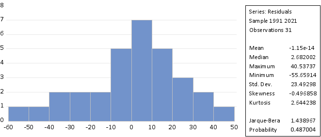
4.10.2. Tests for Normality
The normality test was carried out in the study using the Jarque-Bera, test with a result of 1.438967 (
figure 1), and a probability value of 0.487004 which is greater than 5 percent. This suggests that the above research model used is normally distributed.
Figure 1. Normality Test results.
Source: Author’s computations and Eviews output
*Approximate p-values do not account for coefficient estimation
Source: Authors’ Computation and EViews 13. Outp
4.10.3. Heteroscedasticity Test
From the results of the heteroskedasticity tests conducted using Breusch-Pagan-Godfrey PBG obtained the Obs * R-squared amounted to 7.567467 and the Pro. Chi-Square (2) 0.1817 greater than 5 percent, this can be concluded that there was no heteroscedasticity from the study model (Table 11).
Table 11. Heteroscedasticity Test Results.
F-statistic | 1.6106 | Prob. F(5,26) | 0.1924 |
Obs*R-squared | 7.5675 | Prob. Chi-Square(5) | 0.1817 |
Scaled explained SS | 3.6971 | Prob. Chi-Square(5) | 0.5938 |
Source: Authors’ Computation and EViews 13. Output
4.10.4. Multicollinearity Test
From the results in
Table 12, it can be seen that the Centered VIF value is less than 10, so it can be concluded that in the regression model, there is no multicollinearity and the regression model is feasible to use.
Table 12. Multicollinearity Test Results.
Variable | Coefficient | Uncentered | Centered |
Variance | VIF | VIF |
D_LNREER | 0.017216 | 1.078172 | 1.04361 |
D_LNDISCR | 0.067731 | 1.495142 | 1.435523 |
D_LNINF | 0.0913 | 1.48043 | 1.385471 |
D_LNM2 | 0.034495 | 1.486046 | 1.448712 |
C | 0.154657 | 14.59008 | NA |
Source: Authors’ Computation and EViews 13. Output
5. Conclusion and Recommendations
The premise of this study has been to examine the effect of real effective exchange rate movement on coffee export growth for the period of 1991 to 2022. The study utilized the Vector Error Correction(VECM) to explore this effects of explanatory variables on coffee export growth.
This notwithstanding, before the model was estimated; the properties of the variables (parameters) were established in terms of stationarity and long-run relationship. The Augmented Dickey-Fuller (ADF) test for stationarity and the Johannsson co-integration test for long-run relationship were conducted. The study finds that REER has an enormous positive relationship on coffee export growth in the long run. A unit increase in depreciation of the Tanzanian shillings against the USD results in increases in the coffee export growth by approximately 0.9489 percentage points.
The results from the study show that the depreciation of the domestic currency influences coffee demand in the rest of the world, thus leading to an increase in export volume and revenue which helps to foster coffee export growth.
Inflation and money supply variations are also seen to have a negative and significant relationship with coffee export growth in the long run which signifying that, inflation and money supply determine coffee export growth in the long-run, however in the short –run this relationship is not statistically significant at 5% level.
Finally, having done the very necessary test, and analysis required of this study work; the study concludes by recommending that, it is imperative for Tanzania’s monetary policy authority to carefully monitor exchange rate fluctuations and implement appropriate monetary policy strategies to manage the risks that may happen on coffee exports growth associating with currency movement.
Abbreviations
ADF: Augmented Dickey-Fuller
ARDL: Auto-Regressive Distributed Lag
BOT: Bank of Tanzania various reports
CEG: Coffee Export Growth
DISCR: Discount Rate
GDP: Gross Domestic Product
ICO: International Coffee organization and
INF: Inflation
REER: Real Effective Exchange Rate
TCB: Tanzania Coffee Board,
TZS: Tanzanian shillings
USD: United State Dollar
VECM: Vector Error Correlation Model
Author Contributions
Raphael Mbunduki is the sole author. The author read and approved the final manuscript.
Conflicts of Interest
The author declares no conflicts of Interest.
References
| [1] |
Athanasius, N. (2017). An analysis of banks’ credit and agricultural output in Nigeria: 1980-2014. International Journal of Innovative Finance and Economic Research 5(1), 54, 66.
|
| [2] |
Elias, A., Dachito, A., & Abdulbari, S. (2023). The effects of currency devaluation on Ethiopia’s major export commodities: The case of coffee and khat: Evidence from the vector error correction model and the Johansen co-integration test. Cogent Economics & Finance, 11(1), 2184447.
|
| [3] |
Chambers, R. G., & Just, R. E. (1982). An investigation of the effect of monetary factors on China’s food industry.
|
| [4] |
Devadoss, S. (1985). The impacts of monetary policies on US agriculture (United States).
|
| [5] |
Dushmanitch, V. Y., and Darroch, M. A. G. (1990). An economic analysis of the impacts of monetary policy on South African agriculture.
|
| [6] |
FAO (2020); Production Quantity Data.
|
| [7] |
George, W. (2022). Export performance of the horticultural sub-sector in Tanzania. In Trade and Investment in East Africa (pp. 293-313). Springer, Singapore.
|
| [8] |
Granger, C. W., & Newbold, P. (1974). Spurious regressions in econometrics. Journal of econometrics, 2(2), 111-120.
|
| [9] |
Hong, T. T. K. (2016). Effects of exchange rate and world prices on the export price of Vietnamese coffee. International Journal of Economics and Financial Issues, 6(4), 1756-1759.
|
| [10] |
International coffee organization “Annual report”. Available from
http://www.ico.org/prices/pr-prices.pdf
(ath; [Accessed 12 November 2023])
|
| [11] |
Iliyasu, A. S. (2019). An empirical analysis of the impact of interest rates on agriculture is the exchange rate is the culprit. Federal Reserve Bank of St. Louis Review, Journal of Social Sciences, 5(1), 613.
|
| [12] |
Kargbo, J. M. (2006). Exchange rate volatility and agricultural trade under policy reform in South Africa. Development Southern Africa, 23(01), 147-170.
|
| [13] |
Lechuga Montenegro, J., & Vega Miranda, F. (2018). The impact of interest and exchange rates on Mexican agricultural exports: a study for the period 1993-2017. Textual: análisis del medio rural latinoamericano, (72), 125-149.
|
| [14] |
Mao, R. (2019). Exchange rate effects on agricultural exports: A firm-level investigation of China’s food industry
|
| [15] |
Marwa, N. (2019). Unlocking Coffee Production in Tanzania: What Does the Future Holds. Policy Brief, (7).
|
| [16] |
Mehare, A., & Edriss, A. K. (2013). Evaluation of the Effect of Exchange Rate Variability on the Export of Ethiopia’s Agricultural Product: A Case of Coffee. Margin: The Journal of Applied Economic Research, 7(2), 171–183.
https://doi.org/10.1177/0973801013483506
|
| [17] |
Mlay, N. (2020). Assessing the Effect of Agricultural Export Values on Foreign Exchange Rate in Tanzania
|
| [18] |
Moh’d, A. V. (2020). The effect of exchange rate, inflation rate, interest rate and economic growth on agriculture export earnings in Tanzania
|
| [19] |
Rutashoborwa, P. M. H. (2013). Impact of International Trade on Coffee Industry: The Case of Kagera Region in North-West Tanzania
|
| [20] |
Samoei, S. K., & Kipchoge, E. K. (2021). Drivers of Horticultural Exports in Kenya. Journal of Economics and Financial Analysis, 4(2), 27-44.
|
| [21] |
Schuh, G. E. (1974). The exchange rate and US agriculture. American Journal of Agricultural. Economics, 56(1), 1-13.
|
| [22] |
Shane, M., Roe, T., & Somwaru, A. (2008). Exchange rates, foreign income, and US
|
| [23] |
Tanzania Coffee Board “(2020) Available from
https://Coffee.go.tz
[Accessed 16 March 2023]
|
| [24] |
Tumaini, H. D. (2018). Influence of Exchange Rate Volatility on coffee exports in Tanzania from 1996 to 2016 (Doctoral dissertation, The Open University of Tanzania).
|
| [25] |
Udeaja, E. A., & Elijah, U. A. (2014). Effect of monetary policy on the agricultural sector in Nigeria.
|
Cite This Article
-
-
@article{10.11648/j.ijae.20240902.18,
  author = {Raphael Mbunduki},
  title = {Effects of Exchange Rate Variability on Coffee Export Growth in Tanzania
},
  journal = {International Journal of Agricultural Economics},
  volume = {9},
  number = {2},
  pages = {120-133},
  doi = {10.11648/j.ijae.20240902.18},
  url = {https://doi.org/10.11648/j.ijae.20240902.18},
  eprint = {https://article.sciencepublishinggroup.com/pdf/10.11648.j.ijae.20240902.18},
  abstract = {Exchange rate movement is perceived as a very important factor in influencing the performance of the agriculture sector. When the currency of the exporting country depreciates against the trading partners’ currencies tends to stimulate demand and improve export earnings. An increase in value of the currency against the other trading partners’ currencies (e.g. USD) tend to affect the costs of production that may affect aggregate agricultural supply. However, the linkage of the exchange rate and agricultural export growth in particular traditional exports such as coffee has never been properly and intensively documented for appropriate decision-making in Tanzania. Therefore, this study was set to assess how exchange rate variability has affected coffee export growth in Tanzania. The study made use of time series data from 1991 to 2022 using the vector error collection model (VECM). Given the influences other than the real effective exchange rate on the export of coffee growth, we discriminately incorporated inflation rate, discount rate, and money supply, as the independent variables. Yearly data (1991-2022) obtained from the Bank of Tanzania and the International Coffee Organization were used for the analysis. The results from this study reveal that the real effective exchange rate has an enormous positive impact on coffee export growth in the long run. This implies that, the depreciation of the domestic currency against USD has advantage on coffee export growth when considering the demand side as it tends to stimulate coffee demand in the rest of the world, thus leading to an increase in export volume and revenue which helps to foster coffee export growth. However, in the supply side, this depreciation should be carefully monitored as excess depreciation may end up by rising inputs prices especially those inputs imported such as fertilizers, agrochemical, aggrotech and agro machineries that may intern affect the production level. The study ends by concluding, that it is imperative for the Central Bank to carefully observer exchange rate fluctuations and implement appropriate monetary policy strategies in favour of the agriculture sector in particular exportable crops such as coffee. This will help to manage the risks and opportunities that may arise in coffee export growth associated with currency movement.
},
 year = {2024}
}
 Copy
|
Copy
|
 Download
-
TY  - JOUR
T1  - Effects of Exchange Rate Variability on Coffee Export Growth in Tanzania

AU  - Raphael Mbunduki
Y1  - 2024/04/29
PY  - 2024
N1  - https://doi.org/10.11648/j.ijae.20240902.18
DO  - 10.11648/j.ijae.20240902.18
T2  - International Journal of Agricultural Economics
JF  - International Journal of Agricultural Economics
JO  - International Journal of Agricultural Economics
SP  - 120
EP  - 133
PB  - Science Publishing Group
SN  - 2575-3843
UR  - https://doi.org/10.11648/j.ijae.20240902.18
AB  - Exchange rate movement is perceived as a very important factor in influencing the performance of the agriculture sector. When the currency of the exporting country depreciates against the trading partners’ currencies tends to stimulate demand and improve export earnings. An increase in value of the currency against the other trading partners’ currencies (e.g. USD) tend to affect the costs of production that may affect aggregate agricultural supply. However, the linkage of the exchange rate and agricultural export growth in particular traditional exports such as coffee has never been properly and intensively documented for appropriate decision-making in Tanzania. Therefore, this study was set to assess how exchange rate variability has affected coffee export growth in Tanzania. The study made use of time series data from 1991 to 2022 using the vector error collection model (VECM). Given the influences other than the real effective exchange rate on the export of coffee growth, we discriminately incorporated inflation rate, discount rate, and money supply, as the independent variables. Yearly data (1991-2022) obtained from the Bank of Tanzania and the International Coffee Organization were used for the analysis. The results from this study reveal that the real effective exchange rate has an enormous positive impact on coffee export growth in the long run. This implies that, the depreciation of the domestic currency against USD has advantage on coffee export growth when considering the demand side as it tends to stimulate coffee demand in the rest of the world, thus leading to an increase in export volume and revenue which helps to foster coffee export growth. However, in the supply side, this depreciation should be carefully monitored as excess depreciation may end up by rising inputs prices especially those inputs imported such as fertilizers, agrochemical, aggrotech and agro machineries that may intern affect the production level. The study ends by concluding, that it is imperative for the Central Bank to carefully observer exchange rate fluctuations and implement appropriate monetary policy strategies in favour of the agriculture sector in particular exportable crops such as coffee. This will help to manage the risks and opportunities that may arise in coffee export growth associated with currency movement.

VL  - 9
IS  - 2
ER  -
Copy
|
Download