Rainfall is essential in hydrologic and hydraulic analyses, serving as critical parameter in water resource studies. Hydraulic structures are designed to manage flooding triggered by extreme rainfall events. One common approach to analyze these extreme occurrences is through probability distribution or frequency analysis. This study evaluates various methods of rainfall frequency analysis. Rainfall data was sourced from the Ethiopian Meteorological Agency (EMA), specifically the Addis Ababa Observatory. Before conducting frequency analyses, data quality was assessed for outliers, with findings within acceptable limits. The frequency analysis utilizes four different distribution methods: Gumbel Extreme Value I, Lognormal, Pearson II and Log-Pearson III. Moreover, these distribution methods were fitted using RMC BestFit software to select a method that fits best for the dataset. The fitted distribution methods were also calibrated with non-probability Intensity-Duration-Frequency (IDF) models. Results indicated that while all methods performed satisfactorily, the Gumbel EVI displayed the best balance between model fit and error reduction in this IDF analysis. The study underscores the importance of selecting appropriate statistical methods for accurate rainfall modeling, which is vital for the design and operation of hydraulic structures. Future research could investigate the applicability of these findings in other regions or integrate climate change variables into rainfall frequency analysis for enhanced flood risk management. Additionally, employing advanced techniques, like machine learning algorithms, may improve prediction accuracy and provide deeper understanding of rainfall variability and trends.
| Published in | Hydrology (Volume 14, Issue 1) |
| DOI | 10.11648/j.hyd.20261401.11 |
| Page(s) | 1-14 |
| Creative Commons |
This is an Open Access article, distributed under the terms of the Creative Commons Attribution 4.0 International License (http://creativecommons.org/licenses/by/4.0/), which permits unrestricted use, distribution and reproduction in any medium or format, provided the original work is properly cited. |
| Copyright |
Copyright © The Author(s), 2026. Published by Science Publishing Group |
Addis Ababa, Rainfall, Frequency Analysis, IDF, Gumbel EVI
Location | Data period | Duration | Total record | Format | Unit | ||
|---|---|---|---|---|---|---|---|
Easting = 38°45′ | Northing = 9°1′ | Start year = 1980 | End year = 2018 | 24 hour (daily) | 39 year | Table | mm |
year | Maximum rainfall record | year | Maximum rainfall record | year | Maximum rainfall record |
|---|---|---|---|---|---|
1980 | 36.3 | 1993 | 53.5 | 2006 | 70.9 |
1981 | 58.0 | 1994 | 57.0 | 2007 | 64.0 |
1982 | 41.4 | 1995 | 85.3 | 2008 | 53.3 |
1983 | 50.1 | 1996 | 67.0 | 2009 | 54.7 |
1984 | 55.4 | 1997 | 46.3 | 2010 | 44.6 |
1985 | 43.2 | 1998 | 78.3 | 2011 | 55.8 |
1986 | 83.8 | 1999 | 37.4 | 2012 | 36.4 |
1987 | 56.8 | 2000 | 37.1 | 2013 | 47.2 |
1988 | 35.5 | 2001 | 42.5 | 2014 | 65.4 |
1989 | 49.2 | 2002 | 29.5 | 2015 | 33.1 |
1990 | 39.6 | 2003 | 46.2 | 2016 | 47.7 |
1991 | 47.3 | 2004 | 44.2 | 2017 | 50.8 |
1992 | 51.4 | 2005 | 58.6 | 2018 | 55.2 |
Measure | Record Length | Minimum | Maximum | Mean | Std Dev | Skewness | Kurtosis | Mean (of log) | Std Dev (of log) | Skewness (of log) | Kurtosis (of log) |
|---|---|---|---|---|---|---|---|---|---|---|---|
Value | 39 | 30 | 85 | 52 | 13 | 0.8252 | 0.6051 | 1.6989 | 0.1081 | 0.1721 | -0.1354 |
Skewness coefficient | >+0.4 | <-0.4 | Between ±0.4 |
|---|---|---|---|
Test for | Higher outliers | Lower outlier | Both high and low outliers |
 and
and  are high and low outlier threshold in log units respectively, kn = coefficient depends on sample size (for N = 39; kn = 2.671)
 T | 2 | 5 | 10 | 25 | 50 | 100 |
|---|---|---|---|---|---|---|
KT | -0.16436 | 0.719822 | 1.305225 | 2.044883 | 2.593603 | 3.138272 |
Test method | Value | Remark | |
|---|---|---|---|
Outlier | Higher from test | 97.3 | Ok |
Upper limit from the data | 85.3 | ||
Lower from test | 25.7 | Ok | |
Lower limit from the data | 29.5 | ||
Duration (min) | 5 | 10 | 15 | 20 | 30 | 45 | 60 | 90 | 120 | 180 | 240 | 720 | 1440 |
|---|---|---|---|---|---|---|---|---|---|---|---|---|---|
t(hr) | 0.08 | 0.17 | 0.25 | 0.33 | 0.50 | 0.75 | 1.00 | 1.50 | 2.00 | 3.00 | 4.00 | 12.00 | 24.00 |
b+24 | 24.30 | 24.30 | 24.30 | 24.30 | 24.30 | 24.30 | 24.30 | 24.30 | 24.30 | 24.30 | 24.30 | 24.30 | 24.30 |
(b+24)n | 19.75 | 19.75 | 19.75 | 19.75 | 19.75 | 19.75 | 19.75 | 19.75 | 19.75 | 19.75 | 19.75 | 19.75 | 19.75 |
b+t | 0.38 | 0.47 | 0.55 | 0.63 | 0.80 | 1.05 | 1.30 | 1.80 | 2.30 | 3.30 | 4.30 | 12.30 | 24.30 |
(b+t)n | 0.41 | 0.49 | 0.57 | 0.65 | 0.81 | 1.05 | 1.28 | 1.73 | 2.18 | 3.05 | 3.91 | 10.45 | 19.75 |
RRt | 0.17 | 0.28 | 0.36 | 0.42 | 0.51 | 0.59 | 0.64 | 0.71 | 0.76 | 0.81 | 0.84 | 0.95 | 1.00 |
Probability distribution | Frequency factor, KT for different return periods | |||||
|---|---|---|---|---|---|---|
2 | 5 | 10 | 25 | 50 | 100 | |
Gumbel EVT-I | -0.164 | 0.7195 | 1.304563 | 2.0438 | 2.5923 | 3.137 |
Log Normal | -1.01E-07 | 0.8415 | 1.281729 | 1.7511 | 2.0542 | 2.327 |
Pearson III | -0.135 | 0.7743 | 1.333730 | 1.9981 | 2.4663 | 2.915 |
Log Pearson III | -0.029 | 0.8319 | 1.298620 | 1.8089 | 2.1455 | 2.453 |
Distribution | AIC | BIC | RMSE |
|---|---|---|---|
Gumbel (EVI) | 310.49 | 313.48 | 1.85 |
Log-Normal | 310.64 | 313.64 | 2.23 |
Log-Pearson Type III | 312.77 | 317.07 | 1.98 |
Pearson Type III | 312.52 | 316.82 | 1.98 |
No. | IDF models | R2 | MSE | |
|---|---|---|---|---|
1 | Gumbel EVT-I | I = | 0.9705 | 71.88 |
3 | Log Normal | I = | 0.9703 | 70.35 |
4 | Pearson III | I = | 0.9702 | 71.77 |
5 | Log Pearson III | I = | 0.9704 | 72.00 |
AACRA | Addis Ababa City Road Authority |
AIC | Akaike Information Criteria |
BIC | Bayesian Information Criteria |
DDF | Depth Duration Frequency |
EMA | Ethiopian Meteorological Agency |
ERA | Ethiopia Road Authority |
EVI | Extreme Value I |
GRG | Generalized Reduced Gradient |
IIDF | Intensity-Duration-Frequency |
LP | Linear Programming |
MLE | Maximum Likelihood Estimation |
Probability Density Function | |
RMC | Risk Management Center |
RMSE | Root Mean Square Error |
Rainfall intensity (mm/hr) | ||||||||||||
|---|---|---|---|---|---|---|---|---|---|---|---|---|
5 min | 10 min | 15 min | 20 min | 30 min | 45 min | 60 min | 90 min | 120 min | 180 min | 240 min | 720 min | 1440 min |
14.34 | 23.86 | 30.69 | 35.86 | 43.24 | 50.30 | 54.92 | 60.77 | 64.43 | 68.96 | 71.79 | 80.61 | 85.30 |
14.08 | 23.44 | 30.15 | 35.23 | 42.48 | 49.41 | 53.96 | 59.70 | 63.30 | 67.75 | 70.52 | 79.19 | 83.80 |
13.16 | 21.90 | 28.17 | 32.92 | 39.69 | 46.17 | 50.41 | 55.78 | 59.14 | 63.30 | 65.90 | 74.00 | 78.30 |
11.92 | 19.83 | 25.51 | 29.81 | 35.94 | 41.80 | 45.65 | 50.51 | 53.55 | 57.32 | 59.67 | 67.00 | 70.90 |
11.26 | 18.74 | 24.10 | 28.17 | 33.96 | 39.51 | 43.14 | 47.73 | 50.61 | 54.16 | 56.39 | 63.32 | 67.00 |
10.99 | 18.29 | 23.53 | 27.50 | 33.15 | 38.56 | 42.11 | 46.59 | 49.40 | 52.87 | 55.04 | 61.81 | 65.40 |
10.76 | 17.90 | 23.03 | 26.91 | 32.44 | 37.74 | 41.21 | 45.60 | 48.34 | 51.74 | 53.86 | 60.48 | 64.00 |
9.85 | 16.39 | 21.08 | 24.64 | 29.70 | 34.55 | 37.73 | 41.75 | 44.26 | 47.37 | 49.32 | 55.38 | 58.60 |
9.75 | 16.22 | 20.87 | 24.38 | 29.40 | 34.20 | 37.34 | 41.32 | 43.81 | 46.89 | 48.81 | 54.81 | 58.00 |
9.58 | 15.94 | 20.51 | 23.96 | 28.89 | 33.61 | 36.70 | 40.61 | 43.05 | 46.08 | 47.97 | 53.87 | 57.00 |
9.55 | 15.89 | 20.44 | 23.88 | 28.79 | 33.49 | 36.57 | 40.47 | 42.90 | 45.92 | 47.80 | 53.68 | 56.80 |
9.38 | 15.61 | 20.08 | 23.46 | 28.28 | 32.90 | 35.93 | 39.75 | 42.15 | 45.11 | 46.96 | 52.73 | 55.80 |
9.31 | 15.49 | 19.93 | 23.29 | 28.08 | 32.67 | 35.67 | 39.47 | 41.85 | 44.79 | 46.62 | 52.36 | 55.40 |
9.28 | 15.44 | 19.86 | 23.21 | 27.98 | 32.55 | 35.54 | 39.33 | 41.70 | 44.63 | 46.46 | 52.17 | 55.20 |
9.19 | 15.30 | 19.68 | 23.00 | 27.73 | 32.25 | 35.22 | 38.97 | 41.32 | 44.22 | 46.03 | 51.69 | 54.70 |
8.99 | 14.96 | 19.25 | 22.49 | 27.12 | 31.55 | 34.45 | 38.11 | 40.41 | 43.25 | 45.02 | 50.56 | 53.50 |
8.96 | 14.91 | 19.18 | 22.41 | 27.02 | 31.43 | 34.32 | 37.97 | 40.26 | 43.09 | 44.86 | 50.37 | 53.30 |
8.64 | 14.38 | 18.49 | 21.61 | 26.05 | 30.31 | 33.09 | 36.62 | 38.82 | 41.55 | 43.26 | 48.58 | 51.40 |
8.54 | 14.21 | 18.28 | 21.36 | 25.75 | 29.95 | 32.71 | 36.19 | 38.37 | 41.07 | 42.75 | 48.01 | 50.80 |
8.42 | 14.01 | 18.02 | 21.06 | 25.40 | 29.54 | 32.26 | 35.69 | 37.84 | 40.50 | 42.16 | 47.35 | 50.10 |
8.27 | 13.76 | 17.70 | 20.68 | 24.94 | 29.01 | 31.68 | 35.05 | 37.16 | 39.77 | 41.41 | 46.50 | 49.20 |
8.02 | 13.34 | 17.16 | 20.05 | 24.18 | 28.13 | 30.71 | 33.98 | 36.03 | 38.56 | 40.14 | 45.08 | 47.70 |
7.95 | 13.23 | 17.02 | 19.89 | 23.98 | 27.89 | 30.45 | 33.70 | 35.73 | 38.24 | 39.81 | 44.70 | 47.30 |
7.93 | 13.20 | 16.98 | 19.84 | 23.93 | 27.83 | 30.39 | 33.63 | 35.65 | 38.16 | 39.72 | 44.61 | 47.20 |
7.78 | 12.95 | 16.66 | 19.47 | 23.47 | 27.30 | 29.81 | 32.99 | 34.97 | 37.43 | 38.97 | 43.76 | 46.30 |
7.77 | 12.92 | 16.62 | 19.42 | 23.42 | 27.24 | 29.75 | 32.91 | 34.90 | 37.35 | 38.88 | 43.66 | 46.20 |
7.50 | 12.47 | 16.05 | 18.75 | 22.61 | 26.30 | 28.72 | 31.77 | 33.69 | 36.06 | 37.53 | 42.15 | 44.60 |
7.43 | 12.36 | 15.90 | 18.58 | 22.40 | 26.06 | 28.46 | 31.49 | 33.39 | 35.73 | 37.20 | 41.77 | 44.20 |
7.26 | 12.08 | 15.54 | 18.16 | 21.90 | 25.47 | 27.81 | 30.78 | 32.63 | 34.92 | 36.36 | 40.83 | 43.20 |
7.14 | 11.89 | 15.29 | 17.87 | 21.54 | 25.06 | 27.36 | 30.28 | 32.10 | 34.36 | 35.77 | 40.16 | 42.50 |
6.96 | 11.58 | 14.89 | 17.41 | 20.99 | 24.41 | 26.66 | 29.49 | 31.27 | 33.47 | 34.84 | 39.12 | 41.40 |
6.66 | 11.08 | 14.25 | 16.65 | 20.07 | 23.35 | 25.50 | 28.21 | 29.91 | 32.01 | 33.33 | 37.42 | 39.60 |
6.29 | 10.46 | 13.46 | 15.72 | 18.96 | 22.05 | 24.08 | 26.64 | 28.25 | 30.24 | 31.48 | 35.34 | 37.40 |
6.24 | 10.38 | 13.35 | 15.60 | 18.81 | 21.88 | 23.89 | 26.43 | 28.02 | 29.99 | 31.22 | 35.06 | 37.10 |
6.12 | 10.18 | 13.10 | 15.30 | 18.45 | 21.46 | 23.44 | 25.93 | 27.49 | 29.43 | 30.63 | 34.40 | 36.40 |
6.10 | 10.15 | 13.06 | 15.26 | 18.40 | 21.40 | 23.37 | 25.86 | 27.42 | 29.35 | 30.55 | 34.30 | 36.30 |
5.97 | 9.93 | 12.77 | 14.92 | 17.99 | 20.93 | 22.86 | 25.29 | 26.81 | 28.70 | 29.88 | 33.55 | 35.50 |
5.56 | 9.26 | 11.91 | 13.92 | 16.78 | 19.52 | 21.31 | 23.58 | 25.00 | 26.76 | 27.86 | 31.28 | 33.10 |
4.96 | 8.25 | 10.61 | 12.40 | 14.95 | 17.39 | 18.99 | 21.02 | 22.28 | 23.85 | 24.83 | 27.88 | 29.50 |
Return Period | 2 | 5 | 10 | 25 | 50 | 100 |
|---|---|---|---|---|---|---|
Duration (min.) | Rainfall Intensity (mm/hr) | Rainfall Intensity (mm/hr) | Rainfall Intensity (mm/hr) | Rainfall Intensity (mm/hr) | Rainfall Intensity (mm/hr) | Rainfall Intensity (mm/hr) |
5 | 99.57 | 123.13 | 138.72 | 158.43 | 173.05 | 187.56 |
10 | 82.84 | 102.44 | 115.42 | 131.81 | 143.98 | 156.05 |
15 | 71.04 | 87.85 | 98.98 | 113.04 | 123.47 | 133.83 |
20 | 62.27 | 77.00 | 86.75 | 99.07 | 108.21 | 117.29 |
30 | 50.05 | 61.89 | 69.73 | 79.63 | 86.98 | 94.27 |
45 | 38.81 | 47.99 | 54.07 | 61.75 | 67.45 | 73.11 |
60 | 31.79 | 39.31 | 44.28 | 50.58 | 55.24 | 59.88 |
90 | 23.45 | 28.99 | 32.67 | 37.31 | 40.75 | 44.17 |
120 | 18.64 | 23.06 | 25.98 | 29.67 | 32.40 | 35.12 |
180 | 13.30 | 16.45 | 18.53 | 21.17 | 23.12 | 25.06 |
240 | 10.39 | 12.84 | 14.47 | 16.53 | 18.05 | 19.57 |
720 | 3.89 | 4.81 | 5.42 | 6.19 | 6.76 | 7.32 |
1440 | 2.06 | 2.54 | 2.87 | 3.27 | 3.57 | 3.87 |
Return Period | 2 | 5 | 10 | 25 | 50 | 100 |
|---|---|---|---|---|---|---|
Duration (min.) | Rainfall Intensity (mm/hr) | Rainfall Intensity (mm/hr) | Rainfall Intensity (mm/hr) | Rainfall Intensity (mm/hr) | Rainfall Intensity (mm/hr) | Rainfall Intensity (mm/hr) |
5 | 100.82 | 124.31 | 138.71 | 155.90 | 168.11 | 179.92 |
10 | 83.88 | 103.43 | 115.41 | 129.71 | 139.87 | 149.69 |
15 | 71.94 | 88.70 | 98.97 | 111.24 | 119.95 | 128.37 |
20 | 63.05 | 77.74 | 86.74 | 97.49 | 105.13 | 112.51 |
30 | 50.68 | 62.48 | 69.72 | 78.36 | 84.50 | 90.43 |
45 | 39.30 | 48.46 | 54.07 | 60.77 | 65.53 | 70.13 |
60 | 32.19 | 39.68 | 44.28 | 49.77 | 53.67 | 57.44 |
90 | 23.74 | 29.27 | 32.66 | 36.71 | 39.59 | 42.37 |
120 | 18.88 | 23.28 | 25.97 | 29.19 | 31.48 | 33.69 |
180 | 13.47 | 16.61 | 18.53 | 20.83 | 22.46 | 24.04 |
240 | 10.52 | 12.97 | 14.47 | 16.26 | 17.54 | 18.77 |
720 | 3.94 | 4.85 | 5.42 | 6.09 | 6.56 | 7.03 |
1440 | 2.08 | 2.57 | 2.87 | 3.22 | 3.47 | 3.72 |
Return Period | 2 | 5 | 10 | 25 | 50 | 100 |
|---|---|---|---|---|---|---|
Duration (min.) | Rainfall Intensity (mm/hr) | Rainfall Intensity (mm/hr) | Rainfall Intensity (mm/hr) | Rainfall Intensity (mm/hr) | Rainfall Intensity (mm/hr) | Rainfall Intensity (mm/hr) |
5 | 100.35 | 124.59 | 139.50 | 157.21 | 169.69 | 181.64 |
10 | 83.49 | 103.66 | 116.06 | 130.80 | 141.18 | 151.13 |
15 | 71.60 | 88.90 | 99.54 | 112.17 | 121.08 | 129.60 |
20 | 62.75 | 77.91 | 87.24 | 98.31 | 106.12 | 113.59 |
30 | 50.44 | 62.62 | 70.12 | 79.02 | 85.29 | 91.30 |
45 | 39.12 | 48.56 | 54.38 | 61.28 | 66.14 | 70.80 |
60 | 32.04 | 39.77 | 44.53 | 50.19 | 54.17 | 57.99 |
90 | 23.63 | 29.34 | 32.85 | 37.02 | 39.96 | 42.77 |
120 | 18.79 | 23.33 | 26.12 | 29.44 | 31.78 | 34.01 |
180 | 13.41 | 16.65 | 18.64 | 21.00 | 22.67 | 24.27 |
240 | 10.47 | 13.00 | 14.55 | 16.40 | 17.70 | 18.95 |
720 | 3.92 | 4.86 | 5.45 | 6.14 | 6.63 | 7.09 |
1440 | 2.07 | 2.57 | 2.88 | 3.25 | 3.51 | 3.75 |
Return Period | 2 | 5 | 10 | 25 | 50 | 100 |
|---|---|---|---|---|---|---|
Duration (min.) | Rainfall Intensity (mm/hr) | Rainfall Intensity (mm/hr) | Rainfall Intensity (mm/hr) | Rainfall Intensity (mm/hr) | Rainfall Intensity (mm/hr) | Rainfall Intensity (mm/hr) |
5 | 100.10 | 124.02 | 139.29 | 158.16 | 171.98 | 185.65 |
10 | 83.29 | 103.18 | 115.89 | 131.59 | 143.08 | 154.46 |
15 | 71.43 | 88.49 | 99.39 | 112.85 | 122.71 | 132.47 |
20 | 62.60 | 77.55 | 87.11 | 98.90 | 107.54 | 116.10 |
30 | 50.32 | 62.33 | 70.01 | 79.50 | 86.44 | 93.32 |
45 | 39.02 | 48.34 | 54.30 | 61.65 | 67.03 | 72.37 |
60 | 31.96 | 39.59 | 44.47 | 50.49 | 54.90 | 59.27 |
90 | 23.57 | 29.20 | 32.80 | 37.24 | 40.50 | 43.72 |
120 | 18.74 | 23.22 | 26.08 | 29.62 | 32.20 | 34.76 |
180 | 13.37 | 16.57 | 18.61 | 21.13 | 22.98 | 24.80 |
240 | 10.44 | 12.94 | 14.53 | 16.50 | 17.94 | 19.37 |
720 | 3.91 | 4.84 | 5.44 | 6.18 | 6.72 | 7.25 |
1440 | 2.07 | 2.56 | 2.88 | 3.27 | 3.55 | 3.84 |
| [1] | AACRA. (2004). Urban Road Drainage Precipitation. In Addis Ababa City Road Authority Drainage Design Manual. Addis Ababa City Road Authority, Addis Ababa; Ethiopia. |
| [2] | Agakpe, M. D., Nyatuame, M., & Ampiaw, F. (2024). Development of intensity - duration - frequency (IDF) curves using combined rain gauge (RG) and remote sense (TRMM) datasets for Weta Traditional Area in Ghana. HydroResearch, 7, 109-121. |
| [3] | Agza, M., Assefa, A., & Legeta, B. (2025). Advancement of Intensity Duration Frequency (IDF) Curve Through Possible Probability Distribution Method Using Disaggregated Precipitation Data; The Case of Wolkite, Ethiopia. American Journal of Water Science and Engineering, 11(2), 30-39. |
| [4] | Amona, T., & Worajo, W. E. (2022). Developing Maximum Intensity Duration Frequency (IDF)Curve to WolaitaSodo City, Ethiopia. Journal of University of Shanghai for Science and Technology, 24(5), 62-76. |
| [5] | Basumatary, V., & Sil, B. S. (2016). Generation of Rainfall Intensity-Duration-Frequency curves for the Barak River Basin. Meteorology Hydrology and Water Management., 6, 47-57. |
| [6] | Chow, V. Te, Maidment, D. R., & Mays, L. W. (1988). Applied Hydrology. In Applied Catalysis (Vol. 132). McGraw-Hill. |
| [7] | de Paola, F., Giugni, M., Topa, M. E., & Bucchignani, E. (2014). Intensity-Duration-Frequency (IDF) rainfall curves, for data series and climate projection in African cities. SpringerPlus, 3(1), 1-18. |
| [8] | El Adlouni, S., & Ouarda, T. B. M. J. (2013). Frequency Analysis of Extreme Rainfall Events. Rainfall: State of the Science, January 2010, 171-188. |
| [9] | Ena, G., Alvaro, L., Mart, L., Medrano-barboza, J. P., Freddy, J., Remolina, L., Seingier, G., Walter, L., & L, A. A. (2020). Case Study : Depth-Duration Ratio in a Semi-Arid Zone in Mexico. MDPI (Hydrology). |
| [10] | ERA. (2013). Ethiopia Road Authority Drainage design manual. |
| [11] | Gámez-Balmaceda, E., López-Ramos, A., Martínez-Acosta, L., Medrano-Barboza, J. P., López, J. F. R., Seingier, G., Daesslé, L. W., & López-Lambraño, A. A. (2020). Rainfall intensity-duration-frequency relationship. Case study: Depth-duration ratio in a semi-arid zone in Mexico. Hydrology, 7(4), 1-22. |
| [12] | Gnecco, I., Palla, A., La Barbera, P., Roth, G., & Giannoni, F. (2023). Defining intensity-duration-frequency curves at short durations: a methodological framework. Hydrological Sciences Journal, 68(11), 1499-1512. |
| [13] |
Haden Smith, & Doughty, M. (2020). RMC-BestFit Quick Start Guide.
https://www.publications.usace.army.mil/Portals/76/EM5-1-11_Project Delivery Business Process_2024 0830.pdf |
| [14] | KGomathy, C., Bala Narasimha Reddy, A., Pavan Kumar, A., & LOKESH Sri Chandrasekharendra SaraswathiViswa Mahavidyalaya, A. (2021). a Study on Rainfall Prediction Techniques. International Journal of Scientific Research in Engineering and Management, December. |
| [15] | Lettenmaier, D. (2024). Role of Rainfall in Hydrological Modeling and Water Resource Planning. Citation: Lettenmaier D, 14(1000319), 1000319-1000320. |
| [16] | Mbajiorgu, C. C. (2015). Development of Intensity Duration Frequency (IDF) Curve for Parts of Eastern Catchments Using Modern Arcview GIS Model. January 2012. |
| [17] | Nwaogazie, I. L., & Sam, M. G. (2019). Probability and non-probability rainfall intensity- duration-frequency modeling for Port-Harcourt metropolis, Nigeria. 3(1). |
| [18] | Sandoval, C., Gironás, J., & Chadwick, C. (2025). A Framework for the Assessment of Rainfall Disaggregation Methods in Representing Extreme Precipitation. June, 1-28. |
| [19] |
Selase, A. E., Agyimpomaa, D. E. E., Selasi, D. D., & Hakii, D. M. N. (2015). Precipitation and Rainfall Types with Their Characteristic Features. Journal of Natural Sciences Research, 5(20), 89-92.
https://www.iiste.org/Journals/index.php/JNSR/article/view/26509 |
| [20] | Subramanya, K. (2018). Engineering Hydrology (3rd ed.). Tata McGraw-Hill. |
| [21] | Sun, Y., Wendi, D., Kim, D. E., & Liong, S. Y. (2019). Deriving intensity-duration-frequency (IDF) curves using downscaled in situ rainfall assimilated with remote sensing data. Geoscience Letters, 6(1). |
| [22] | Thanh, S. T., & Xuan, A. H. (2023). Deriving of Intensity- Duration- Frequency (IDF) curves for precipitation at Hanoi, Vietnam. E3S Web of Conferences, 403. |
| [23] | Van de Vyver, H., & Demarée, G. R. (2010). Elaboration des courbes Intensité-Durée-Fréquence (IDF) des précipitations à Lubumbashi, Congo, sous l’hypothèse des données insuffisantes. Hydrological Sciences Journal, 55(4), 555-564. |
| [24] | Venkatacharyulu, S., Sreeram, V., Rajashekhar, T., Bindu, K. H., Joshi, A., & Mittal, V. (2025). Rainfall Frequency Analysis and Urban Flood Modelling. AIP Conference Proceedings, 3157(1). |
| [25] | Vischel, T., & Panthou, G. (2018). Technical notes on Intensity-duration-frequency curves for the city of Ouagadougou : A tool for helping with the dimensioning of hydraulic structures. 1-6. |
| [26] | Wambua, R. M. (2019). Estimating Rainfall Intensity-Duration-Frequency (Idf) Curves For A Tropical River Basin. 3(4), 99-106. |
| [27] | Yong, S. L. S., Ng, J. L., Yuk Feng Huang, & Ang, C. K. (2021). ASSESSMENT OF THE BEST PROBABILITY DISTRIBUTION METHOD IN RAINFALL. Malaysian Journal Of Civil Engineering, 1, 16253. |
APA Style
Agza, M. D. (2026). A Methodological Comparison of Rainfall Frequency Distribution Derived from Disaggregated Rainfall Records. Hydrology, 14(1), 1-14. https://doi.org/10.11648/j.hyd.20261401.11
ACS Style
Agza, M. D. A Methodological Comparison of Rainfall Frequency Distribution Derived from Disaggregated Rainfall Records. Hydrology. 2026, 14(1), 1-14. doi: 10.11648/j.hyd.20261401.11
@article{10.11648/j.hyd.20261401.11,
  author = {Mezen Desse Agza},
  title = {A Methodological Comparison of Rainfall Frequency Distribution Derived from Disaggregated Rainfall Records},
  journal = {Hydrology},
  volume = {14},
  number = {1},
  pages = {1-14},
  doi = {10.11648/j.hyd.20261401.11},
  url = {https://doi.org/10.11648/j.hyd.20261401.11},
  eprint = {https://article.sciencepublishinggroup.com/pdf/10.11648.j.hyd.20261401.11},
  abstract = {Rainfall is essential in hydrologic and hydraulic analyses, serving as critical parameter in water resource studies. Hydraulic structures are designed to manage flooding triggered by extreme rainfall events. One common approach to analyze these extreme occurrences is through probability distribution or frequency analysis. This study evaluates various methods of rainfall frequency analysis. Rainfall data was sourced from the Ethiopian Meteorological Agency (EMA), specifically the Addis Ababa Observatory. Before conducting frequency analyses, data quality was assessed for outliers, with findings within acceptable limits. The frequency analysis utilizes four different distribution methods: Gumbel Extreme Value I, Lognormal, Pearson II and Log-Pearson III. Moreover, these distribution methods were fitted using RMC BestFit software to select a method that fits best for the dataset. The fitted distribution methods were also calibrated with non-probability Intensity-Duration-Frequency (IDF) models. Results indicated that while all methods performed satisfactorily, the Gumbel EVI displayed the best balance between model fit and error reduction in this IDF analysis. The study underscores the importance of selecting appropriate statistical methods for accurate rainfall modeling, which is vital for the design and operation of hydraulic structures. Future research could investigate the applicability of these findings in other regions or integrate climate change variables into rainfall frequency analysis for enhanced flood risk management. Additionally, employing advanced techniques, like machine learning algorithms, may improve prediction accuracy and provide deeper understanding of rainfall variability and trends.},
 year = {2026}
}
TY  - JOUR
T1  - A Methodological Comparison of Rainfall Frequency Distribution Derived from Disaggregated Rainfall Records
AU  - Mezen Desse Agza
Y1  - 2026/04/07
PY  - 2026
N1  - https://doi.org/10.11648/j.hyd.20261401.11
DO  - 10.11648/j.hyd.20261401.11
T2  - Hydrology
JF  - Hydrology
JO  - Hydrology
SP  - 1
EP  - 14
PB  - Science Publishing Group
SN  - 2330-7617
UR  - https://doi.org/10.11648/j.hyd.20261401.11
AB  - Rainfall is essential in hydrologic and hydraulic analyses, serving as critical parameter in water resource studies. Hydraulic structures are designed to manage flooding triggered by extreme rainfall events. One common approach to analyze these extreme occurrences is through probability distribution or frequency analysis. This study evaluates various methods of rainfall frequency analysis. Rainfall data was sourced from the Ethiopian Meteorological Agency (EMA), specifically the Addis Ababa Observatory. Before conducting frequency analyses, data quality was assessed for outliers, with findings within acceptable limits. The frequency analysis utilizes four different distribution methods: Gumbel Extreme Value I, Lognormal, Pearson II and Log-Pearson III. Moreover, these distribution methods were fitted using RMC BestFit software to select a method that fits best for the dataset. The fitted distribution methods were also calibrated with non-probability Intensity-Duration-Frequency (IDF) models. Results indicated that while all methods performed satisfactorily, the Gumbel EVI displayed the best balance between model fit and error reduction in this IDF analysis. The study underscores the importance of selecting appropriate statistical methods for accurate rainfall modeling, which is vital for the design and operation of hydraulic structures. Future research could investigate the applicability of these findings in other regions or integrate climate change variables into rainfall frequency analysis for enhanced flood risk management. Additionally, employing advanced techniques, like machine learning algorithms, may improve prediction accuracy and provide deeper understanding of rainfall variability and trends.
VL  - 14
IS  - 1
ER  -
Department of Hydraulic and Water Resources Engineering, Wolkite University, Wolkite, Ethiopia
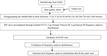
Figure 1. Graphical representation of IDF model development.
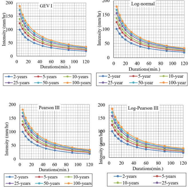
Figure 2. Intensity Distribution Frequency Curves of different distribution method.
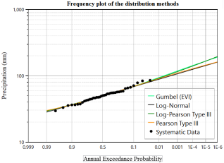
Figure 3. Different distribution method frequency plot in comparison with the station data.
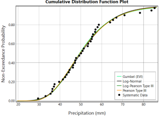
Figure 4. Cumulative distribution plot of different distribution methods.
Information

