Research Article | | Peer-Reviewed

An Explanation for the Existence of Stall Hysteresis

Received: 20 November 2024     Accepted: 20 December 2024     Published: 10 February 2025
Views:       Downloads:
Abstract

An explanation of the mechanism for the difference in angle for separation and reattachment during stall on airfoils via potential flow and stall-prediction theories is proposed as follows: the reattachment angle of any given airfoil is the stall angle of the effective body which encompasses the physical body and its trailing viscous wake. Airfoil hysteresis exists, above certain Reynolds numbers, when the angle of attack increases beyond the catastrophic stall angle with the flow remaining separated until lowered below the stall angle of attack. The size of the hysteresis loop is determined by the difference in separation and reattachment angles. Within the clockwise hysteresis loop there exist two distinct airfoil geometries: the physical and the effective. The physical, or actual airfoil geometry, dominates the behavior of the pre-catastrophic lift. The much longer (relatively thinner) effective body dominates the hysteresis loop from catastrophic stall to reattachment, which is what the flow “sees” from the potential flow perspective. Wind tunnel tests were conducted at the United States Air Force Academy’s (USAFA’s) Sub-Sonic Wind Tunnel (SWT) where excellent agreement (less than half a degree) is found for all tests thus far.

Published in Fluid Mechanics (Volume 10, Issue 1)
DOI 10.11648/j.fm.20251001.11
Page(s) 1-10
Creative Commons

This is an Open Access article, distributed under the terms of the Creative Commons Attribution 4.0 International License (http://creativecommons.org/licenses/by/4.0/), which permits unrestricted use, distribution and reproduction in any medium or format, provided the original work is properly cited.

Copyright

Copyright © The Author(s), 2025. Published by Science Publishing Group

Keywords

Stall, Hysteresis, Airfoil, Aerodynamics, Fluid Mechanics, Flight Mechanics, Flow Control, Stall Hysteresis

1. Introduction
Stall hysteresis, and its mechanism, are open questions within aerodynamics being investigated physically and numerically . Pilot intervention, due to the difference between the stall and reattachment angles, often requires pushing the nose down significantly to reattach flow and resume flying and / or to avoid spin entry . For wind turbine blades, the dynamics of stall hysteresis notably contributes to blade fatigue and reduced operational life . Similar reasons exist to control hysteresis on compressor blades today as well as historically . Whether interested in prolonging machine or human lifespans, how to either avoid or control stall hysteresis is of high importance to the aerodynamic community. This work proposes to answer the how-hysteresis-arises question.
Hysteresis refers to how the current state of a system depends on the earlier, or historical state of the system. For flow around a wing or airfoil, a given flow state (attached or separated) depends on whether the flow was attached or separated previously. A typical lift curve with hysteresis, as in the Reynolds number dependent data in Figure 1 , can, for a given angle of attack (α), have more than one associated lift coefficient. It should be stated that a flow can experience a mix of attached and separated flow, however, we will refer to either an attached state or a stalled/separated state.
Aerodynamicists are familiar with the maximum lift point of the stall angle. In Figure 1, the blue triangle at the peak of the lift curve (~10° - 11°) is the stall angle. There is also the “catastrophe angle” marked by the red circle in Fig 1. Once at a post-catastrophic angle, the lowering of the angle of attack to the pre-catastrophic angle does not result in an attached state.
To illustrate, using the Re =168 k series in Figure 1, if the angle of attack is increased from 10° to 13°, the lift coefficient decreases marginally from just above 1.3 to just below 1.3. If the angle of attack is then lowered back to 10°, the lift coefficient will return to the value at the lower angle – in other words, just above 1.3. Instead, if increasing the angle from 13° to 15° the coefficient of lift will drop from 1.3 to 0.75. Now, lowering the angle of attack from 15° to 10° the lift coefficient will stay at 0.75 and not the pre-catastrophic state of above 1.3. In short, the stalled flow field persists until the angle of attack is decreased enough. Additionally, given that an immediate lowering of angle of attack once stall is fully developed, will not result in a reattached state, this is not a time-dependent phenomenon – it is purely a function of geometry.
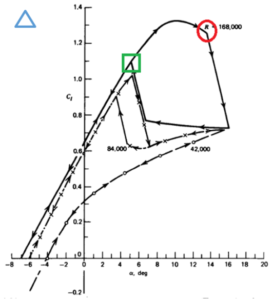
Figure 1. Stall hysteresis at multiple Reynolds number for N60 airfoil . The blue triangle was originaly at the peak in the curve.
This function of geometry also holds true at what we call the “reattachment angle” – the green square on the hysteresis loop in Figure 1. If the flow is already fully stalled, and the angle of attack is lowered enough (to the green square) causing reattachment, an immediate increase to the previous angle of attack will not result in stalled conditions – the attached state now dominates the flow field. Extending the previous illustration, lowering the angle of attack to around 5°, from 10°, the flow reattaches near this lower angle with an attendant increase in lift to ~1.1. However, if the angle increases again to 10°, the lift coefficient will increase to ~1.3+ as the flow is in an attached-dominated state.
The opportunity to prolong human and machine life through understanding and controlling the hysteresis loop hinges on the notion of decreasing the angle of attack enough.
The same trend can be seen in Figure 2 , with a Reynolds number = 47 5k for a NACA 0012 airfoil. The blue (up pointing triangles) line is the ascending trend line with a clear catastrophic angle near 13°. The orange (down pointing triangles) line depicts the trend while decreasing angle of attack and indicates that flow does not reattach until ~11°, at which point the lift produced by the airfoil will once again follow the blue (ascending) trend line.
Figure 2. Stall Hysteresis of NACA 0012 at Re = 475 k .
1.1. Potential Flow
An airfoil at a low angle of attack is shown in Figure 3 with the associated viscous boundary layer and effective body (not to scale). Potential flow theory yields reasonably accurate lift force predictions for a physical body (PB) when the boundary layer and surrounding viscous wake are included together as a single effective body (EB) . At low angles of attack the EB is essentially a scaled-up model of the physical body in thickness and chord. In fact, it is this EB the potential flow experiences as the boundary layer height is the extent of viscous and rotational effects. In other words, potential flow conditions exist outside the boundary layer .
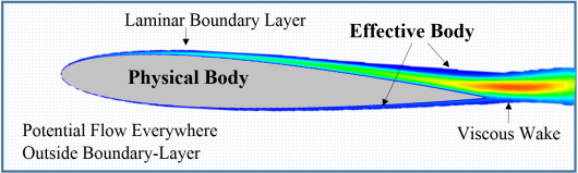
Figure 3. Effective body and potential flow.
A similar situation exists at higher, even post-stall, angles of attack. Increasingly sophisticated modifications to potential flow methods, through the process of decambering , have been made by modifying the airfoil geometry via a decrease in camber as the angle of attack is increased. Potential-flow decambering-techniques rely on existing lift curves to match empirical results. These methods show excellent agreement on the non-linear portion of the lift curve up to stall and very good agreement to mildly post-stall angles.
A potential-flow effective body also exists at post-catastrophic angles. However, in this case, the effective body is much longer than the physical body and has some negative camber owing to the trailing viscous wake and high angle of attack. The potential flow goes around the effective body (region of viscosity/vorticity) as though it were a physical structure. Afterall, the trailing wake is of higher pressure than the outer potential flow, otherwise the wake would collapse. This is shown qualitatively in Figure 4, where there is a wake of darker to lighter blue (slower flow / higher pressure) trailing the NACA 0012 (the physical body, black) and experiencing a shear with the outer potential flow (lighter green). Figure 5 shows an outline of the effective body (EB) for a post-stalled airfoil, which is elongated in contrast to the low angle of attack case in Figure 3.
Note how the chord length of the EB increases. The trailing edge of an EB will inevitably come down to a judgement-call on where the boundary between the inner-flow (boundary layer) and the outer (potential) flow is. Practically speaking, this is identical to defining the height of the boundary layer. Is it at 95%U or 99.5% U? In other words, the choice of boundary value has little effect on macroscopic behavior while still being useful.
We postulate the post-catastrophic reattachment-angle of the physical body is governed by the separated flow. Therefore, for this investigation, instead of matching the lift curve values of the physical body (Figure 2) via a decambering or other method, we attempt to match the effective body geometry of the post-catastrophic flow-field (Figures 4 and 5) to test how it behaves.
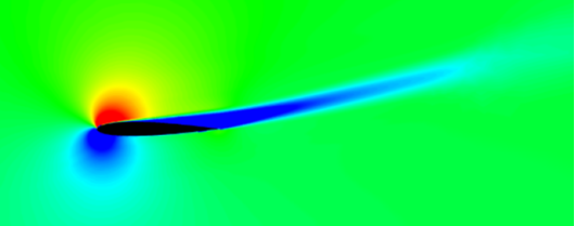
Figure 4. X-velocity contour of a NACA 0012 at 15.5⁰ Re = 475 k. Qualitatively, where Green is the freestream, Blue is slower, and Red is faster. .
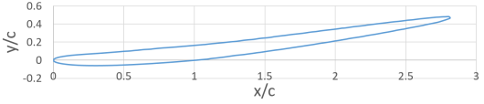
Figure 5. Effective body of a stalled airfoil .
1.2. Hysteresis Hypothesis
The present hypothesis is as follows: the reattachment angle for a given physical airfoil is the stall angle of the associated effective body (e.g. Figure 5). That is to say, a stalled flow field persists, despite lowering the angle of attack below the ascending catastrophe or stall angle, until the angle of attack is lowered below the effective body’s stall angle. Only then can the flow reattachment occur. Otherwise, if the angle remains above the reattachment angle, the potential flow continues around the effective body – the expanded boundary layer and wake of the physical body. However, once reattachment occurs, the stalled flow field is convected away, the effective body shrinks back to just larger than the physical body (as in Figure 3), and the lift behavior returns to the ascending curves seen in Figures 1 and 2.
2. Methodology
A multi-pronged approach was taken for this investigation utilizing wind tunnels as well as CFD resources. Models of physical bodies were printed with metal spars and were run through angle of attack sweeps in the wind tunnel to obtain Cl vs a curves to determine the stall, catastrophe, and reattachment angles for a given geometry and Reynolds number. Simultaneously, CFD of the physical bodies were run at tunnel conditions to determine the shape of the effective body. Once determined, the effective bodies were printed and run in the same manner as the physical body models with the stall angle being of primary interest to support or refute the hysteresis hypothesis: the reattachment angle of the PB is the stall angle of the associated EB.
Although implied previously, it should be explicitly stated that we are discussing static stall hysteresis. There are no pitch rates or α̇ in this study. Hence the prior statement regarding no time dependence. Each model was positioned to a given angle of attack for some period and the average force recorded (and coefficients calculated) following a “settling time” of 2 – 3 seconds (or longer for post-stall). Clearly, flows near stall are inherently unsteady. What is meant by “settling time” is such that the transient of the change of angle of attack has passed and any behavior left (whether steady or unsteady) is a function of the new angle of attack for the given flow parameters, so called asymptotically steady.
2.1. Model
The geometry for the physical bodies was the prosaic NACA0012. These were 3D printed in sections, mounted on a steel spar, end-plates installed, glued together, and surface prepped for the tunnel . The CFD procedure to determine the effective body geometry is described below in Section III.2. However, once that geometry was determined, EB models were constructed (section 3.2) in the same manner as the PB models (Figure 6).
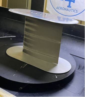
Figure 6. NACA 3406 (analog for NACA0012EB) mounted in USAFA SWT.
2.2. Experimental Setup
Tests were initially undertaken at the Doryland wind tunnel at ERAU with following tests at the FluiDyne subsonic wind tunnel (SWT) located inside the USAFA aero lab . At ERAU, the model was mounted to a sting-balance. At USAFA, the model (airfoil, endplates, and beam) was vertically placed inside the Ate-Ltd external balance in the spanwise-center of the tunnel. The balance is capable of sampling forces at 4.8 kHz (forwarding data packets at 400 Hz). While the external balance can measure a total of six axes of force and moment, side force was the primary measurand due to the airfoil orientation and sole requirement to determine lift coefficient. Due to near continuous use, both tunnel and instrumentation are regularly calibrated. Tests were run on the PB from Re = 300 k to 1.0 M and for the EB from Re = 750 k to 2.7 M at subsonic Mach numbers (M = 0.15 – 0.23) to avoid compressibility effects.
2.3. Procedure
Following a warmup procedure, the tunnel was brought to the desired Reynolds number conditions. The angle of attack of the model was increased until the airfoil was confidently past its stall angle and then lowered again. A total of ten runs per condition, including an inverted test, were performed as a repeatability study. Table 1 shows the maximum uncertainty in the measured quantities.
Table 1. Maximum uncertainty in measurements.

Measurand

Bias

Percent of Full Scale

Angle of Attack

±.05°

.0025%

Coefficient of Lift

±.00838

.036%

Reynolds Number

±13530

1.01%

3. Results & Discussion
3.1. Physical Body Results from Re = 0.3 M to 0.5 M
Low speed wind tunnel testing revealed a positive correlation between lift-curve hysteresis and Reynolds number. As Reynolds number was increased, the stall angle was observed to increase by 2.5°, the reattachment angle however grew by less than 1°, resulting in a set of expanding hysteresis loops, as can be seen in Figures 7-10 [21]. Note that each data marker in the following figures (as well as Figure 2) is large enough to encompass the maximum extent of experimental error along the linear portion of the curve.
Each of these figures has the typical linear lift-curve slope, departing from linear as it approaches the peak lift or stall angle, followed by catastrophic stall while increasing angle of attack. Once the angle of attack is again reduced, we observe the lower lift values (separated state) for a given angle of attack compared with the ascending angle of attack. Note Figure 7 barely demonstrates a hysteresis loop (~1/4°), indicating the Re of 300 k on the NACA0012 is near the boundary for such phenomena.
In Figures 8-10 the hysteresis loop is more evident; a reattachment angle of 11.5° for the case of Re = 4.75 x 10⁵ in Figure 10 is observed.
Figure 7. NACA 0012 at Re = 300 k, M = 0.02.
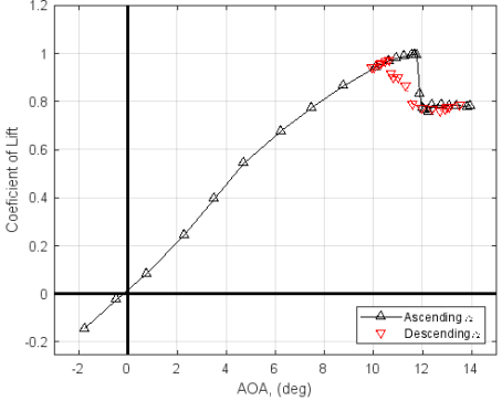
Figure 8. NACA 0012 at Re = 350 k, M = 0.02.
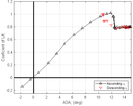
Figure 9. NACA 0012 at Re = 400 k, M = 0.03.
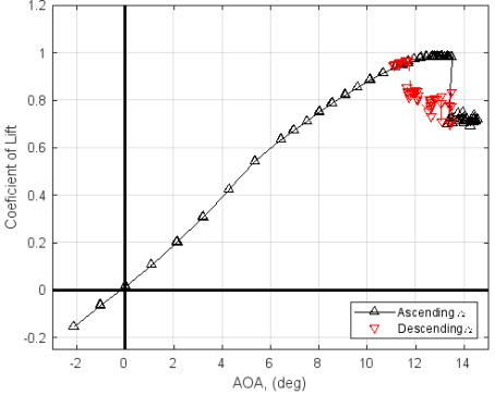
Figure 10. NACA 0012 at Re = 475 k, M = 0.03, reattachment angle ~ 11.5°.
The largest hysteresis loop was captured at Re = 475 k, measuring 2.0⁰. As hysteresis loop size indicates the size of the corresponding effective body, this freestream condition was selected for subsequent numerical experiments.
3.2. Determining the Effective Body
The CFD to determine the effective bodies was undertaken in ANSYS FLUENT using a RANS-SA model (despite the initially lower Reynolds numbers) specifically to achieve an average shape to the viscous wake trailing the physical body (NACA0012). Typical mesh refinement studies were undertaken and are referenced in . The computational models were run through an angle of attack sweep matching the wind tunnel Cl vs a curves giving confidence to the mesh and the model parameters.
Analysis was conducted to simulate the flow field around the NACA 0012 at α = 15.5⁰ for the Re=475 k case as it was approximately 1.0-1.5⁰ beyond the post-catastrophe angle of attack for the initial Reynolds number range under consideration (Re ~1/2 M to 1 M). For post-catastrophe angles, it is expected the effective body will lengthen to some maximum, and that the thickness would also increase. However, as the angle of attack is lowered again, the EB will shrink to some post-catastrophe minimum, the one that persists while lowering angle of attack to the reattachment angle.
These tests were used to identify a region of separated flow extending approximately 3c behind the leading edge, as can be qualitatively seen from the velocity contours shown in Figure 4, and quantitatively in Figure 12.
The effective body, defined by the lower surface of the physical body and the edge of the separated boundary layer, can be identified using the contour of minimum shear stress. Since the flow is incompressible, this minimum-shear layer coincides with the contour where the local dynamic pressure normalized by the freestream dynamic pressure (q/q∞) approaches 1 from the lower bound. To identify the effective body, contours of dynamic pressure were plotted using data from numerical simulations. The contour where q/q∞ = 0.95 was selected to represent the minimum shear layer, shown in Figure 11.
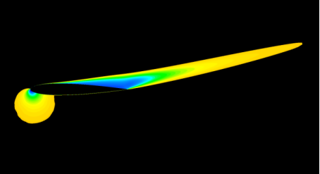
Figure 11. Pressure contour clipped at 0.95q∞.
It should be noted that the circular leading-edge protrusion visible in Figure 11, though part of the relevant pressure contour, is not a part of the boundary-layer and is therefore removed for an accurate representation of the minimum shear layer. The resultant shape, depicted by the red outline in Figure 12, is the effective body for a stalled NACA 0012 at this Reynolds number. This effective body is longer, and therefore has lower relative thickness, with some negative camber, when compared to the NACA 0012 (the white area from 0<x/c<1). Additionally, and of importance for this investigation, the Effective Body being longer has a proportionally higher Reynolds number due to the longer chord. In the case of Figure 12, the EB Reynolds number based on chord is ~2.7 that of the PB or 1.3 M.
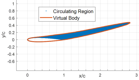
Figure 12. Effective body of a NACA 0012.
The effective body was run at Reynolds numbers from 300 k to 1.0 M. Due to a structural failure of the model during stall at Re = 1 M, the highest Reynolds number for reliable data to this point was 750 k with a stall angle of ~10° (Figure 13). The target Reynolds number of the effective body for the NACA0012 at Re = 475 k (Figure 10) was 1.3 M. This difference in Reynolds number from 750 k to 1.3 M is expected to increase stall angle by approximately 1.5° . Therefore, the stall angle for the effective body at Re = 1.3 M is predicted to be 11.5°, which matches the data in Figure 10.
Before moving on to the following section, which describes EB Reynolds number 1.3 M results, it should be noted that Figure 7 above shows the NACA0012 at Re = 300 k with a stall angle of 10.75° and a reattachment angle of 10.5°. The Effective Body in Figure 13 has an associated PB Re = 278 k, thus, by the same reasoning as above , we would expect either a slightly higher stall angle on the EB of ~10.0° - 10.5° at the higher Re of 810 k OR a slightly lower reattachment angle than the Re = 300 k case in the range of ~10.0° - 10.5° in Figure 7. In either case, this also shows good agreement with the current hypothesis.
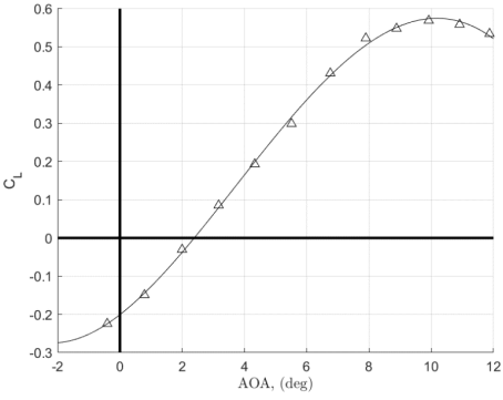
Figure 13. NACA0012EB at Re = 750 k, M = 0.02.
3.3. Analog for the Effective Body and New Structural Model
In Figure 14 we highlight the similarity between the EB gained from CFD analysis in the prior section and an inverted NACA3406. Of note is the fact that the two profiles are nearly identical for 80+% of the chord with the EB geometry being thicker and blunter (not sharp) at the trailing edge compared to the 3406. The similarity between the effective body and the inverted NACA 3406 implies that the stall angles of the two airfoils are similar, if not the same, for a given Reynolds number . The primary purpose in using the analog airfoil was the ability to generate vertex data of any desired resolution for the NACA airfoil versus retooling the code that produced the EB vertices. A close second was the notion that finding historical data for such a close match would aid these investigations – to date, none has come to light.
A model of the inverted NACA3406 profile was printed with an initially 1.5 foot chord and 1.5 foot span with endplates to restrict flow to “2D”. Further, to avoid the failure and loss of another model, a spar made from a 4” x ½” steel bar was used, running full span, to which the endplates were attached. This model was then mounted vertically (See Figure 6) in the USAFA SWT to the force and moment balance. A model of a NACA0012 was made to the same specifications for easy swapping of models during testing. Ultimately, to minimize 3D effects, models with aspects ratios of 2-3 were used.
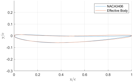
Figure 14. NACA0012EB and inverted NACA 3406.
4. Results and Discussion
4.1. Effective Body Results
Figure 15 is the inverted 3406 (NACA0012EB analog) at Re = 1.3 M. There are two series of data: the first, in blue-open-circles (R1), was taken at every degree, while the second series, in orange-open-squares (R2), was taken at every quarter of a degree. This figure shows the stall angle for the effective body is in the range of 11.0° to 11.25°. It should be noted that the inverted NACA3406 is a “worst-case” or limiting scenario due to its sharp trailing-edge as a blunter trailing geometry would support the flow to slightly higher stall angles .
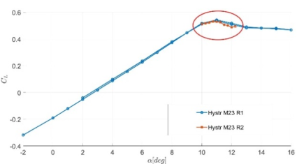
Figure 15. Lift Curve for NACA 0012 Effective Body at Re=1.3 M.
Recalling Figure 10 for a NACA 0012 airfoil showing the full hysteresis loop at a Reynolds number of 475 k. The black line with up-pointing triangles is the ascending trend line with a clear catastrophic stall angle around 13.5°. The red line with down-pointing triangles depicts the trend while decreasing angle of attack and indicates that flow does not reattach until 11.25° to 11.5°, at which point the lift produced by the airfoil will once again follow the black (ascending) trend line whether the angle of attack is increased or decreased – provided the angle of attack is kept below the catastrophic stall angle.
The hysteresis hypothesis states that the reattachment angle of the airfoil will be the stall angle of its attendant effective body. In other words, there is a 0.0° to 0.5° (nominally 1/4°) difference in the measured data of the reattachment angle of the PB to the stall angle of the EB – further supporting the hypothesis.
4.2. Effective Body Results: Higher Reynolds Numbers
The next question of interest is: are these results merely coincidence for the given conditions or would they stand up to further scrutiny such as higher Reynolds numbers or with alternate PB geometries? In answer, the NACA0012 was run at Re = 750 k and 1.0 M through a full hysteresis loop to determine the reattachment angle at those Reynolds numbers. The associated EB Reynolds numbers were 2.0 M and 2.7 M respectively. In Figure 16 is a lift curve for the NACA0012 at Re = 750 k (3/4 M) with upwards-pointing, red-triangles for the ascending angles of attack and the black-bordered, red-squares for the descending angles of attack (post catastrophe). Figure 16 shows the reattachment angle is 14.0° at 750 k for the NACA0012. Similarly, and not shown here, the reattachment angle for Re = 1 M was 14.25°. Both Reynolds numbers were run in the USAFA subsonic wind tunnel at 0.25° steps in the area of stall to capture the hysteresis behavior with reasonable accuracy.
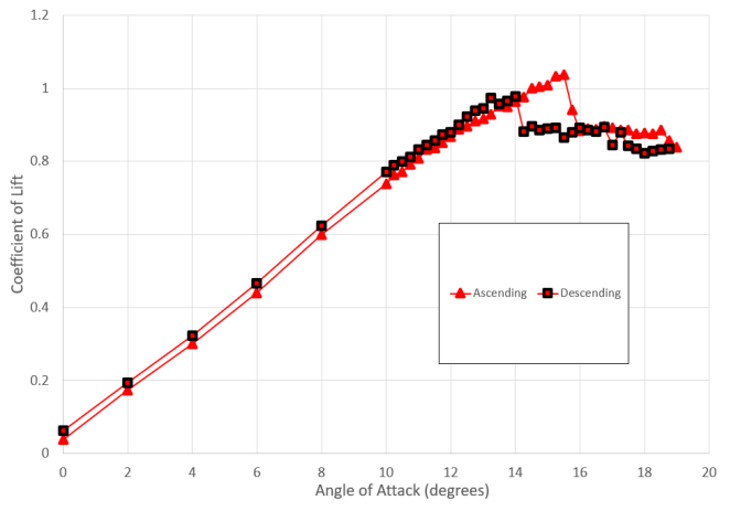
Figure 16. NACA0012 Re= 750 k hysteresis loop.
In Figure 17 there are a pair of runs taken up to 18.0° and back down to 4.0° for the inverted NACA3406 (analog for the NACA0012EB) at Re = 2.025 M, corresponding to the case of the NACA0012 at Re = 3/4 M (750 k). Owing in part to the inverted geometry, and a couple of local maxima in the data, it is difficult to determine where the stall angle for this airfoil is.
The addition of error bars in Figure 18 offers some clarity. First, to ease reading of the figure, note that the error bars were doubled in size. Next, note that while the flow is still attached – while on the linear portion of the curve, the size of the error is relatively “small”. Once the curve departs linear, with the onset and growth of separation, the error grows somewhat.
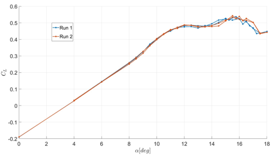
Figure 17. NACA0012EB (3406 inverted) Re= 2.0 M lift curve.
However, once full-on stall occurs, the size of the separation and mixing grow significantly. The error bars grow also given the greater range of values recorded by the force balance. The last “small” error bar occurs at 14.0° (CL +/- 0.025) with a 2.5x increase in that error at 14.5° (CL +/- 0.0625). Hence, the stall angle for the effective body is at 14.25° (+/- 1/4°) – again, matching within a quarter-degree the corresponding reattachment angle of the NACA0012. The results for the inverted NACA3406 (NACA0012EB) at Re = 2.7 M, corresponding to the case of the NACA0012 at Re = 1.0 M were the same. This is not surprising as the stall angle does not change appreciably in this range of Reynolds number .
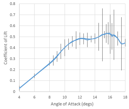
Figure 18. NACA0012EB (3406 inverted) Re= 2.0 M lift curve, stall at 14.0°.
These results further support the hypothesis that the reattachment angle of a given airfoil is the stall angle of the attendant/corresponding effective body (EB). The foregoing results are offered with the following caveat. Following runs of the EB at Re = 2.7 M (PB Re = 1.0 M) testing was discontinued due to potential over-stress concerns for the balance at higher Re and therefore higher tunnel speeds and forces and moments on the balance. It is expected this lack of higher Re data is not a major loss to the community as stall angle tends to converge with increases of Re above a million.
5. Conclusions and Recommendations
A theory describing the underlying mechanism for stall hysteresis is as follows: the reattachment angle for the physical airfoil of the clockwise hysteresis-loop is the stall angle of the associated, potential-flow-based, effective body. Previous works achieved both qualitative and quantitative agreement and support of the hysteresis hypothesis. The current work contributes additional quantitative support by extending the investigation to higher Reynolds numbers.
Convergent behavior seems to exist in the case of Reynolds number. That is, as Reynolds number increases substantially beyond one million, the stall angle ceases to grow appreciably in contrast to how it grows below one million. Therefore, it is suggested there is an upper limit to the reattachment angle for a given geometry.
Future steps/recommendations include running cambered physical bodies in the wind tunnel, as well as thicker and thinner airfoils, to further validate the preceding statement. Additionally, computational models can be run for the foregoing conditions as well as to higher Reynolds numbers that cannot be safely run in a wind tunnel.
Abbreviations

α

Angle of Attack

αs

Stall Angle

c

Chord

Cd

Section Drag Coefficient

CD

Drag Coefficient

Cl

Section Lift Coefficient

CL

Lift Coefficient

Cl max

Section Lift Coefficient at Stall Angle

Cm

Section Pitch-moment Coefficient

CM

Moment Coefficient

EB

Effective Body Geometry

LE

Leading Edge

M

Mach

PB

Physical Body Geometry

q

Dynamic Pressure

q

Free-stream Dynamic Pressure

Re

Reynolds Number

x

Horizontal Distance from LE

y

Vertical Distance from LEr

Acknowledgments
On behalf of my team, I (Morris) would like to thank the NSF for initial funding my efforts, which was incipient to this vein of research. Also, I would like to remember my now passed research advisor and mentor – Dr. Zvi Rusak.
My team of assistants – Grasser, Margiotta, and Wojcik, building on Edwards, Foran, and Pauley, and Stewart and Stoner, and building on Ingraham, Wolfbarger, and Zenker – worked tirelessly in the tunnels and I am indeed grateful for their efforts.
Further I would like to thank DFAN at USAFA and all of the members of the dept and the aero lab that contributed to this project’s success. Specifically, Mr.s Ken Ostasiewski and Tim Siefers.
Finally, I would like to thank DFAN dept chairs: Brigadier General Douglas “Beaker” Wickert, LtCol Dell Olmstead, and LtCol James “Nut” Gresham as well as AFOSR for continuing support of our research.
Author Contributions
Wallace Morris II is the sole author. The author read and approved the final manuscript.
Funding
This work is supported by AFOSR /AFRL seed grant for 2022 and 2023.
Data Availability Statement
The data supporting the outcome of this research work has been reported in this manuscript.
Conflicts of Interest
The authors declare no conflicts of interest.
References
[1] W. J. Morris II & Z. Rusak, “Stall onset on aerofoils at low to moderately high Reynolds number flows,” J. Fluid Mech. (2013), vol. 733, pp. 439-472.
[2] J. J. Bertin & R. M. Cummings “Aerodynamics for Engineers” 6th Ed 2022, Cambridge University Press.
[3] J. Anderson, Fundamentals of Aerodynamics 5th Ed 2011, McGraw-Hill.
[4] W. J. Morris II, S. Stewart, A. Stoner “Wind Tunnel Validation of Stall Hysteresis Hypothesis,” AIAA Aviation (Summer 2022),
[5] Kolin, I. V., Markov, V. G., Trifonova, T. I., “Hysteresis in the static aerodynamic characteristics of a curved-profile wing,” Tech. Phys, Vol. 49, 1 Feb. 2004, pp. 263–266.
[6] Hristov, G., Ansell, P. J., “Poststall Hysteresis and Flowfield Unsteadiness on a NACA 0012 Airfoil. Aerospace Research Central,” 7 July 2018.
[7] Traub, L. W., “Effects of Plain and Gurney Flaps on a Nonslender Delta Wing,” Journal of Aircraft, Vol. 56, No. 2, 2019.
[8] Traub, L. W., “Experimental Investigation of a Morphable Biplane,” Journal of Aircraft, Vol. 49, No. 1, 2012.
[9] Sereez, M., Abramov, N. B., and Goman, M. G., “Prediction of Static Aerodynamic Hysteresis on a Thin Airfoil Using OpenFOAM,” Journal of Aircraft, 13 Oct. 2020,
[10] Mittal, S., and Saxena, P., “Hysteresis in flow past a NACA 0012 Airfoil,” Computer Methods in Applied Mechanics and Engineerings, Vol. 191, Issues 19-20, 1 Mar. 2002.
[11] Khare, A., Singh, A., Nokam, K., “Best Practices in Grid Generation for CFD Applications Using Hypermesh,” Computational Research Laboratories, Pune, Maharashtra, India, 2009.
[12] Rumsey, C. L., Spalart, P. R., “Turbulence Model Behavior in Low Reynolds Number Regions of Aerodynamic Flowfields,” AIAA Journal, Vol. 47, No. 4, 2009.
[13] Z. Yang, H. Igarashi, M. Martin and H. Hu, “An Experimental Investigation on Aerodynamic Hysteresis of a Low-Reynolds Number Airfoil,” AIAA Aerospace Sciences Meeting, AIAA-2008-0315, 2008.
[14] D. Crider & J. Foster, “Simulation Modeling Requirements for Loss-of-Control Accident Prevention of Turboprop Transport Aircraft,” AIAA Modeling and Simulation Technologies Conference, AIAA 2012-4569, 2012.
[15] C. P. Butterfield, A. C. Hansen, D. Simms, G. Scott, “Dynamics Stall on Wind Turbine Blades,” 1991, NREL TP-257-4510.
[16] M. Arjomandi, and R. Kelso, “Estimation of Dynamic Stall on Wind Turbine Blades using an Analytical Model,” 18th Australasian Fluid Mechanics Conference, 2012.
[17] Zhiping LI, Peng ZHANG, Tianyu PAN, Qiushi LI, Jian ZHANG, “Hysteresis behaviors of compressor rotating stall with cusp catastrophic model,” Chinese j. of Aeronautics, May 2018, vol 31, pp. 1075-1084.
[18] A. Mendelson, “Aerodynamic Hysteresis as a Factor in Critical Flutter Speed of Compressor Blades at Stalling Conditions”, J. Aeronautical Sciences, Vol. 16, No. 11 (1949), pp. 645-652.
[19] B. W. McCormick, “Aerodynamics Aeronautics and Flight Mechanics,” Wiley and Sons, second edition, 1995, p.142, figure 3.81.
[20] A. Sherman, “Interference of Wings and Fuselage from Test of 30 Combinations with Triangular and Elliptical Fuselages in the NACA Variable-Density Tunnel”, NACA TN 1272, 1947.
[21] W. J. Morris II, J. Ingraham, T. Wolfenbarger, & C. Zenker “A Hypothesis of Stall Hysteresis - Why the reattachment angle is less than the separation stall angle” AIAA SciTech (January 2020)
[22] Z. Rusak & W. Morris II, “Stall Onset on Airfoils at Moderately High Reynolds Number Flows,” ASME Journal of Fluids Engineering November 1, 2011.
[23] E. Jacobs & A. Sherman, “Airfoil Section Characteristics as Affected by Variations of the Reynolds Number,” NACA TR-586, 1937.
[24] Lighthill, M. J., “On Displacement Thickness,” Journal of Fluid Mechanics, Vol. 4, No. 4, 1958.
[25] Katz, J. and Plotkin, A., Low-Speed Aerodynamics, Cambridge Aerospace Series, Cambridge University Press, Cambridge, UK, 2001. (Lumped Vortex Model).
[26] R. Mukherjee, “Post-Stall Prediction of Multiple-Lifting-Surface Configurations Using a Decambering Approach. (Under the direction of Dr. Ashok Gopalarathnam.)” Ph.D. Dissertation, Aerospace Engineering, North Carolina State University, Raleigh, NC, 2004.
[27] P. Hosangadi and A. Gopalarathnam, “Low-Order Method for Prediction of Separation and Stall on Unswept Wings” J. Aircraft (AIAA), Volume 58, Number 3, May 2021,
[28] I. H Abbott & A. E VonDoenhoff,, “Theory of Wing Sections,” 1958, 2nd Edition, Dover Press.
[29] Anderson, R. F., “The Aerodynamic Characteristics of Airfoils at Negative Angles of Attack,” National Advisory Committee for Aeronautics, Technical Note No. 412, March 1932.
Cite This Article
  • APA Style

    II, W. M. (2025). An Explanation for the Existence of Stall Hysteresis. Fluid Mechanics, 10(1), 1-10. https://doi.org/10.11648/j.fm.20251001.11

    Copy | Download

    ACS Style

    II, W. M. An Explanation for the Existence of Stall Hysteresis. Fluid Mech. 2025, 10(1), 1-10. doi: 10.11648/j.fm.20251001.11

    Copy | Download

    AMA Style

    II WM. An Explanation for the Existence of Stall Hysteresis. Fluid Mech. 2025;10(1):1-10. doi: 10.11648/j.fm.20251001.11

    Copy | Download

  • @article{10.11648/j.fm.20251001.11,
      author = {Wallace Morris II},
      title = {An Explanation for the Existence of Stall Hysteresis},
      journal = {Fluid Mechanics},
      volume = {10},
      number = {1},
      pages = {1-10},
      doi = {10.11648/j.fm.20251001.11},
      url = {https://doi.org/10.11648/j.fm.20251001.11},
      eprint = {https://article.sciencepublishinggroup.com/pdf/10.11648.j.fm.20251001.11},
      abstract = {An explanation of the mechanism for the difference in angle for separation and reattachment during stall on airfoils via potential flow and stall-prediction theories is proposed as follows: the reattachment angle of any given airfoil is the stall angle of the effective body which encompasses the physical body and its trailing viscous wake. Airfoil hysteresis exists, above certain Reynolds numbers, when the angle of attack increases beyond the catastrophic stall angle with the flow remaining separated until lowered below the stall angle of attack. The size of the hysteresis loop is determined by the difference in separation and reattachment angles. Within the clockwise hysteresis loop there exist two distinct airfoil geometries: the physical and the effective. The physical, or actual airfoil geometry, dominates the behavior of the pre-catastrophic lift. The much longer (relatively thinner) effective body dominates the hysteresis loop from catastrophic stall to reattachment, which is what the flow “sees” from the potential flow perspective. Wind tunnel tests were conducted at the United States Air Force Academy’s (USAFA’s) Sub-Sonic Wind Tunnel (SWT) where excellent agreement (less than half a degree) is found for all tests thus far.},
     year = {2025}
    }
    

    Copy | Download

  • TY  - JOUR
    T1  - An Explanation for the Existence of Stall Hysteresis
    AU  - Wallace Morris II
    Y1  - 2025/02/10
    PY  - 2025
    N1  - https://doi.org/10.11648/j.fm.20251001.11
    DO  - 10.11648/j.fm.20251001.11
    T2  - Fluid Mechanics
    JF  - Fluid Mechanics
    JO  - Fluid Mechanics
    SP  - 1
    EP  - 10
    PB  - Science Publishing Group
    SN  - 2575-1816
    UR  - https://doi.org/10.11648/j.fm.20251001.11
    AB  - An explanation of the mechanism for the difference in angle for separation and reattachment during stall on airfoils via potential flow and stall-prediction theories is proposed as follows: the reattachment angle of any given airfoil is the stall angle of the effective body which encompasses the physical body and its trailing viscous wake. Airfoil hysteresis exists, above certain Reynolds numbers, when the angle of attack increases beyond the catastrophic stall angle with the flow remaining separated until lowered below the stall angle of attack. The size of the hysteresis loop is determined by the difference in separation and reattachment angles. Within the clockwise hysteresis loop there exist two distinct airfoil geometries: the physical and the effective. The physical, or actual airfoil geometry, dominates the behavior of the pre-catastrophic lift. The much longer (relatively thinner) effective body dominates the hysteresis loop from catastrophic stall to reattachment, which is what the flow “sees” from the potential flow perspective. Wind tunnel tests were conducted at the United States Air Force Academy’s (USAFA’s) Sub-Sonic Wind Tunnel (SWT) where excellent agreement (less than half a degree) is found for all tests thus far.
    VL  - 10
    IS  - 1
    ER  - 

    Copy | Download

Author Information
  • Department of Aeronautics, United States Air Force Academy, Colorado Springs, USA

    Biography: Wallace Morris II is a professor at the United States Air Force Academy’s Aeronautical Engineering Department. He completed his PhD in Aeronautical Engineering at Rensselaer Polytechnic Institute in 2009, and his Master of Science in Aeronautical Engineering from RPI in 2005. Recognized for his exceptional contributions, Dr. Morris has been honoured with the National Science Foundation’s Graduate Research Fellowship Program. His areas of research interest in basic science are Aerodynamics and Computational Fluid Dynamics as applied to Flow-Control and Aircraft Design.

    Research Fields: Aerodynamics, Fluid Mechanics, Computational Fluid Dynamics, Aerodynamic Design, Aircraft Design