Based on new research, the article presents a formula for determining the potential energy of an earthquake with incorporation of seismic moment and displacement angle values. This formula is new compared to the one derived by the author earlier. The mechanical interpretation of the new formula is provided. Much effort is devoted to determining the values of “stress relief” during strong earthquakes. A formula is derived for determining the values of “stress relief” based on shear modulus and ultimate shear strain of the soil stratum at the epicenters of 44 earthquakes. Also, a methodology is offered to determine energy values of earthquakes with complex structures of surface rupture, as well as areas of deformation zones on Earth’s surface and areas of strong earthquake aftershocks’ locations. New formulas are derived for determining such areas and a comparative analysis is provided with similar formulas by K. Kasahara and T. Dambara.
| Published in | Earth Sciences (Volume 14, Issue 1) |
| DOI | 10.11648/j.earth.20251401.13 |
| Page(s) | 33-48 |
| Creative Commons |
This is an Open Access article, distributed under the terms of the Creative Commons Attribution 4.0 International License (http://creativecommons.org/licenses/by/4.0/), which permits unrestricted use, distribution and reproduction in any medium or format, provided the original work is properly cited. |
| Copyright |
Copyright © The Author(s), 2025. Published by Science Publishing Group |
Earthquake Energy, Seismic Moment, Displacement Angle, Stress Relief, Deformation Areas and Aftershock Locations, Empirical Dependencies
 ,
,  on the entire space of the deformed medium, on both sides of the future rupture caused by the pending earthquake.
  . In parallel, formula (3) can be used to determine the ultimate shear strain and tangential stresses for any points of the deformed medium
  , based on the following formulas:
  . It is shown in
  of the rocks in the Earth’s crust. In seismology and geotechnology, for the upper, near-surface rocks value is accepted as kg/cm2. Assuming that kg/cm2, the last column of Table 1 shows the stress relief values for 44 earthquakes, which are in the range from 2 to 57.5 kg/cm2. The stronger the earthquake, the higher the stress relief values.
  . Our research shows that for the 44 selected earthquakes, mean slip values
  are 1.95-2.08 times smaller than the maximum slip values (Figure 5).
 No. | Country | Earthquake location | Date of earthquake occurrence | Type of slip | Earthquake magnitude | Rupture length , [km] | Rupture depth , [km] | Maximum slip , [m] |
|---|---|---|---|---|---|---|---|---|
1 | USA | Fort Tejon | 09.01.1857 | RL | 8.3 | 297 | 12 | 9.4 |
2 | USA | Owens Valley | 26.03.1872 | RL-N | 8 | 108 | 15 | 11 |
3 | Japan | Nobi | 27.10.1891 | LL | 8 | 80 | 15 | 8 |
4 | Japan | Rikuu | 31.08.1896 | R | 7.2 | 40 | 21 | 4.4 |
5 | USA | San Francisco | 1/13/1906 | RL | 7.8 | 432 | 12 | 6.1 |
6 | USA | Pleasant Valley | 10/3/1915 | N | 7.6 | 62 | 15 | 5.8 |
7 | China | Kansy | 12/16/1920 | LL | 8.5 | 220 | 20 | 10 |
8 | Japan | North Izu | 11/25/1930 | LL- R | 7.3 | 35 | 12 | 3.8 |
9 | China | Kehetuohai | 8/10/1931 | RL | 7.9 | 180 | 20 | 14.6 |
10 | Turkey | Erzincan | 12/26/1939 | RL | 7.8 | 360 | 20 | 7.5 |
11 | USA | Imperial Valley | 5/19/1940 | RL | 7.2 | 60 | 11 | 5.9 |
12 | China | Damxung | 11/18/1951 | RL | 8 | 200 | 10 | 12 |
13 | USA | Dixie Valley | 12/16/1954 | RL-R | 6.8 | 45 | 14 | 3.8 |
14 | Turkey | Abant | 5/26/1957 | RL | 7 | 40 | 8 | 1.65 |
15 | Mongolia | Gobi-Altai | 12/4/1957 | LL | 7.9 | 300 | 20 | 9.6 |
16 | USA | Hebgen Lake | 8/18/1959 | N | 7.6 | 45 | 17 | 6.1 |
17 | Iran | Dasht-e-Bayaz | 8/31/1968 | LL | 7.1 | 110 | 20 | 5.2 |
18 | Turkey | Gediz | 3/28/1970 | N | 7.1 | 63 | 17 | 2.8 |
19 | USA | San Fernando | 2/9/1971 | R-LL | 6.5 | 17 | 14 | 2.5 |
20 | China | Luhuo | 2/6/1973 | LL | 7.3 | 110 | 13 | 3.6 |
21 | Guatemala | Motagua | 2/4/1976 | LL | 7.5 | 257 | 13 | 3.4 |
22 | Turkey | Caldiran | 11/24/1976 | RL | 7.3 | 90 | 18 | 3.5 |
23 | Iran | Bob-Tangol | 12/19/1977 | RL | 5.8 | 14 | 12 | 0.3 |
24 | Greece | Thessaloniki | 6/20/1978 | N | 6.4 | 28 | 14 | 0.22 |
25 | Iran | Tabas-e-Colshan | 9/16/1978 | R | 7.5 | 74 | 22 | 3 |
26 | USA | Homestead Valley | 3/15/1979 | RL | 5.6 | 6 | 4 | 0.1 |
27 | Australia | Cadoux | 6/2/1979 | R | 6.1 | 16 | 6 | 1.5 |
28 | USA | El Centro | 10/15/1979 | RL | 6.7 | 51 | 12 | 0.8 |
29 | Iran | Koli | 11/27/1979 | LL-R | 7.1 | 75 | 22 | 3.9 |
30 | Algeria | El Asman | 10/10/1980 | R | 7.3 | 55 | 15 | 6.5 |
31 | Italy | South Apennines | 11/23/1980 | N | 6.9 | 60 | 15 | 1.15 |
32 | Greece | Corinth | 2/25/1981 | N | 6.4 | 19 | 16 | 1.5 |
33 | Greece | Corinth | 3/4/1981 | N | 6.4 | 26 | 18 | 1.1 |
34 | USA | Borah Peak | 10/28/1983 | N-LL | 7.3 | 33 | 20 | 2.7 |
35 | Algeria | Constantine | 10/27/1985 | LL | 5.9 | 21 | 13 | 0.12 |
36 | Australia | Marryat Creek | 3/30/1986 | R-LL | 5.8 | 13 | 3 | 1.3 |
37 | Greece | Kalamata | 9/13/1986 | N | 5.8 | 15 | 14 | 0.18 |
38 | New Zealand | Edgecumbe | 3/2/1987 | N | 6.6 | 32 | 14 | 2.9 |
39 | USA | Superstition Hills | 11/24/1987 | RL | 6.6 | 30 | 11 | 0.92 |
40 | Australia | Tennant Greek | 1/22/1988 | R | 6.3 | 13 | 9 | 1.3 |
41 | China | Lancand Gengma | 11/6/1988 | RL | 7.3 | 80 | 20 | 1.5 |
42 | Armenia | Spitak | 12/7/1988 | R-RL | 6.8 | 38 | 11 | 2 |
43 | Canada | Ungava | 12/25/1989 | R | 6.3 | 10 | 5 | 2 |
44 | USA | Landers | 6/28/1992 | RL | 7.6 | 62 | 12 | 6 |
No. | Mean slip , [m] | Seismic moment , [dyne*cm] | Value of from (2), [km] | Energy classes (1) | Energy classes (8) | Ultimate shear strain from (12) | Stress relief , kg/cm2 kg/cm2 |
|---|---|---|---|---|---|---|---|
1 | 6.4 | 114.0 | 47 | 16.68 | 16.79 | 1.07 | 53.5 |
2 | 6 | 48.60 | 45 | 16.30 | 16.41 | 1.05 | 52.5 |
3 | 5.04 | 30.24 | 40.25 | 16.06 | 16.17 | 0.98 | 49 |
4 | 2.59 | 10.88 | 27.95 | 15.49 | 15.60 | 0.73 | 36.5 |
5 | 3.3 | 85.54 | 31.5 | 16.44 | 16.54 | 0.82 | 41 |
6 | 2 | 9.300 | 25 | 15.36 | 15.47 | 0.63 | 31.5 |
7 | 7.25 | 159.5 | 51.25 | 16.84 | 16.95 | 1.11 | 55.5 |
8 | 2.9 | 6.090 | 29.5 | 15.26 | 15.37 | 0.77 | 38.5 |
9 | 7.38 | 132.8 | 51.9 | 16.76 | 16.87 | 1.12 | 56 |
10 | 1.85 | 66.60 | 24.25 | 16.19 | 16.30 | 0.60 | 30 |
11 | 1.5 | 4.950 | 22.5 | 15.01 | 15.11 | 0.52 | 26 |
12 | 8 | 80.00 | 65 | 16.55 | 16.66 | 1.15 | 57.5 |
13 | 2.1 | 6.615 | 25.5 | 15.22 | 15.33 | 0.65 | 32.5 |
14 | 0.55 | 0.880 | 17.75 | 13.92 | 14.02 | 0.24 | 12 |
15 | 6.54 | 196.2 | 47.7 | 16.92 | 17.03 | 1.08 | 54 |
16 | 2.14 | 8.186 | 25.7 | 15.32 | 15.42 | 0.65 | 32.5 |
17 | 2.3 | 25.30 | 26.5 | 15.83 | 15.93 | 0.68 | 34 |
18 | 0.86 | 4.605 | 19.3 | 14.80 | 14.91 | 0.35 | 17.5 |
19 | 1.5 | 1.785 | 22.5 | 14.56 | 14.67 | 0.52 | 26 |
20 | 1.3 | 9.295 | 21.5 | 15.24 | 15.34 | 0.47 | 23.5 |
21 | 2.6 | 43.43 | 28 | 16.09 | 16.20 | 0.73 | 36.5 |
22 | 2.05 | 16.61 | 25.25 | 15.62 | 15.73 | 0.64 | 32 |
23 | 0.12 | 0.101 | 15.6 | 12.38 | 12.48 | 0.06 | 3 |
24 | 0.08 | 0.157 | 15.4 | 12.40 | 12.50 | 0.04 | 2 |
25 | 1.5 | 12.21 | 22.5 | 15.39 | 15.50 | 0.52 | 26 |
26 | 0.05 | 0.006 | 15.25 | 10.78 | 10.95 | 0.03 | 1.5 |
27 | 0.5 | 0.240 | 17.5 | 13.32 | 13.42 | 0.22 | 11 |
28 | 0.18 | 0.551 | 15.9 | 13.28 | 13.39 | 0.09 | 4.5 |
29 | 1.2 | 9.900 | 21 | 15.24 | 15.35 | 0.45 | 22.5 |
30 | 1.54 | 6.353 | 22.7 | 15.12 | 15.23 | 0.53 | 26.5 |
31 | 0.64 | 2.880 | 18.2 | 14.49 | 14.61 | 0.28 | 14 |
32 | 0.6 | 0.912 | 18 | 13.97 | 14.07 | 0.26 | 13 |
33 | 0.6 | 1.404 | 18 | 14.16 | 14.26 | 0.26 | 13 |
34 | 0.8 | 2.640 | 19 | 14.53 | 14.64 | 0.33 | 16.5 |
35 | 0.1 | 0.137 | 15.5 | 12.43 | 12.53 | 0.05 | 2.5 |
36 | 0.5 | 0.098 | 17.5 | 12.93 | 13.03 | 0.22 | 11 |
37 | 0.15 | 0.158 | 15.75 | 12.66 | 12.74 | 0.07 | 3.5 |
38 | 1.7 | 3.808 | 23.5 | 14.93 | 15.04 | 0.57 | 28.5 |
39 | 0.54 | 0.891 | 17.5 | 13.92 | 14.03 | 0.24 | 12 |
40 | 0.63 | 0.369 | 18.15 | 13.59 | 13.70 | 0.27 | 13.5 |
41 | 0.7 | 5.600 | 18.5 | 14.81 | 14.92 | 0.30 | 15 |
42 | 1.22 | 2.550 | 21.1 | 14.65 | 14.76 | 0.45 | 22.5 |
43 | 0.8 | 0.200 | 19 | 13.41 | 13.52 | 0.33 | 16.5 |
44 | 2.95 | 10.97 | 29.75 | 15.52 | 15.63 | 0.78 | 39 |
 on rupture middle areas will be about twice as high, so will reach from 4 to 115 kg/cm2. According to Brune
  usually are in the range of 50-100 bar (kg/cm2), with some as low as a few bars and some others as high as a few hundredbars. For the San Francisco earthquake of 1906 (), the stress relief value was estimated by geodetic methods to be 130 bars.
  m/sec), based on synthetic accelerograms of earthquakes with magnitudes of 7.0, 8.0 and 9.0, at the bedding’s base level (depth of 30 m) the design values of
  reach
reach  ,
,  and
and  , respectively, while the stress relief values at kg/cm2 reach 25 kg/cm2 at , 44 kg/cm2 at , and 64 kg/cm2 at .
  , respectively.
  m (measured on-site after the earthquake), vertical component - m, compression component - m, horizontal component m, R=1090, P=530.
 No. earthquake | Country | Earthquake location | Date of the earthquake | Earthquake Magnitude | Length of the gap (km) | Depth of the rupture h (km) | Maximum movement (m) | Average movement (m) |
|---|---|---|---|---|---|---|---|---|
1 | USA | Fort Tejon | 09.01.1857 | 8.3 | 297 | 12 | 9.4 | 6.4 |
2 | USA | Owens Valley | 26.03.1872 | 8 | 108 | 15 | 11 | 6 |
3 | Japan | Nobi | 27.10.1891 | 8 | 80 | 15 | 8 | 5.04 |
4 | Japan | Rikuu | 31.08.1896 | 7.2 | 40 | 21 | 4.4 | 2.59 |
5 | USA | San Francisco | 1/13/1906 | 7.8 | 432 | 12 | 6.1 | 3.3 |
6 | USA | Pleasant Valley | 10/3/1915 | 7.6 | 62 | 15 | 5.8 | 2 |
7 | China | Kansy | 12/16/1920 | 8.5 | 220 | 20 | 10 | 7.25 |
8 | Japan | North Izu | 11/25/1930 | 7.3 | 35 | 12 | 3.8 | 2.9 |
9 | China | Kehetuohai | 8/10/1931 | 7.9 | 180 | 20 | 14.6 | 7.38 |
10 | Turkеy | Erzihcan | 12/26/1939 | 7.8 | 360 | 20 | 7.5 | 1.85 |
11 | USA | Imperial Valley | 5/19/1940 | 7.2 | 60 | 11 | 5.9 | 1.5 |
12 | China | Damxung | 11/18/1951 | 8 | 200 | 10 | 12 | 8 |
13 | Turkеy | Abant | 5/26/1957 | 7 | 40 | 8 | 1.65 | 0.55 |
14 | Mongolia | Gobi-Altai | 12/4/1957 | 7.9 | 300 | 20 | 9.6 | 6.54 |
15 | USA | Hebgen Lake | 8/18/1959 | 7.6 | 45 | 17 | 6.1 | 2.14 |
16 | Iran | Dasht-e-Bayaz | 8/31/1968 | 7.1 | 110 | 20 | 5.2 | 2.3 |
17 | Turkеy | Gediz | 3/28/1970 | 7.1 | 63 | 17 | 2.8 | 0.86 |
18 | China | Luhuo | 2/6/1973 | 7.3 | 110 | 13 | 3.6 | 1.3 |
19 | Guatemala | Motagua | 2/4/1976 | 7.5 | 257 | 13 | 3.4 | 2.6 |
20 | Turkеy | Caldiran | 11/24/1976 | 7.3 | 90 | 18 | 3.5 | 2.05 |
21 | Iran | Tabas-e-Colshan | 9/16/1978 | 7.5 | 74 | 22 | 3 | 1.5 |
22 | Iran | Koli | 11/27/1979 | 7.1 | 75 | 22 | 3.9 | 1.2 |
23 | Algeria | El Asman | 10/10/1980 | 7.3 | 55 | 15 | 6.5 | 1.54 |
24 | USA | Borah Peak | 10/28/1983 | 7.3 | 33 | 20 | 2.7 | 0.8 |
25 | Armenia | Spitak | 12/7/1988 | 7 | 38 | 11 | 2 | 1.22 |
26 | China | Lancand Gengma | 11/6/1988 | 7.3 | 80 | 20 | 1.5 | 0.7 |
27 | USA | Landers | 6/28/1992 | 7.6 | 62 | 12 | 6 | 2.95 |
No. earthquake | The value of according to the formula (2) (km) | Size of the area Q1/1014, to the formula (15), cm2 | Size of the area Q2/1014, to the formula (16), cm2 | Difference in areas Q1-Q2=<i></i>Q/1014, cm2 | Deviations <i></i>Q/Q2 in % | Deviations Q1/Q2 |
|---|---|---|---|---|---|---|
1 | 47 | 3.02 | 2.92 | 0.10 | 3.42 | 1.03 |
2 | 45 | 0.97 | 1.45 | -0.48 | -33.10 | 0.67 |
3 | 40.25 | 0.64 | 1.45 | -0.81 | -55.86 | 0.44 |
4 | 27.95 | 0.22 | 0.22 | 0.00 | 0.00 | 1.00 |
5 | 31.5 | 2.72 | 0.90 | 1.82 | 202 | 3.02 |
6 | 25 | 0.31 | 0.56 | -0.25 | -44.64 | 0.55 |
7 | 51.25 | 2.26 | 4.68 | -2.42 | -51.71 | 0.48 |
8 | 29.5 | 0.21 | 0.28 | -0.07 | -25.00 | 0.75 |
9 | 51.9 | 1.87 | 1.14 | 0.73 | 64.04 | 1.64 |
10 | 24.25 | 1.75 | 0.90 | 0.85 | 94.44 | 1.94 |
11 | 22.5 | 0.27 | 0.22 | 0.05 | 22.73 | 1.23 |
12 | 65 | 2.60 | 1.45 | 1.15 | 79.31 | 1.79 |
13 | 17.75 | 0.14 | 0.14 | 0.00 | 0.00 | 1.00 |
14 | 47.7 | 2.86 | 1.14 | 1.72 | 151 | 2.51 |
15 | 25.7 | 0.23 | 0.56 | -0.33 | -58.93 | 0.41 |
16 | 26.5 | 0.58 | 0.17 | 0.41 | 241 | 3.41 |
17 | 19.3 | 0.24 | 0.17 | 0.07 | 41.18 | 1.41 |
18 | 21.5 | 0.47 | 0.28 | 0.19 | 67.86 | 1.68 |
19 | 28 | 1.44 | 0.45 | 0.99 | 220 | 3.20 |
20 | 25.25 | 0.45 | 0.28 | 0.17 | 60.71 | 1.61 |
21 | 22.5 | 0.33 | 0.45 | -0.12 | -26.67 | 0.73 |
22 | 21 | 0.32 | 0.17 | 0.15 | 88.24 | 1.88 |
23 | 22.7 | 0.25 | 0.28 | -0.03 | -10.71 | 0.89 |
24 | 19 | 0.13 | 0.28 | -0.15 | -54 | 0.46 |
25 | 21.1 | 0.16 | 0.14 | 0.02 | 14.29 | 1.14 |
26 | 18.5 | 0.30 | 0.28 | 0.02 | 7.14 | 1.07 |
27 | 29.75 | 0.37 | 0.56 | -0.19 | -33.93 | 0.66 |
Average value Average value without earthquakes № 5, 14, 16, 19 | 36 | 1.36 | ||||
6.49 | 1.06 | |||||
| [1] | Khachiyan E. Y., Method for determining the potential strain energy stored in the earth before a large earthquake. Science Publishing Group, Earth Sciences, 2013, 10(2), pp. 47-57., |
| [2] | Khachiyan E. Y., On determining of the ultimate strain of earth crust rocks by the value of relative slips on the earth surface after a large earthquake. Science Publishing Group, Earth Sciences, 2016, 5, pp. 111-118, |
| [3] | Khachiyan E. Y., Predicting of the seismogram and accelerogram of strong motions of the soil for an earthquake model considered as an instantaneous rupture of the earth’s surface. Science Publishing Group, Earth Sciences, 2018, 7, pp. 183-201. |
| [4] | Khachiyan E. Y., Analysis of the Values of Ground Displacements, Shear Strains, Velocities and Accelerations, and Response Spectra of Strong Earthquake by Synthetic Accelerograms. Science Publishing Group, Earth Sciences, 2022, 11(5), pp. 327-337, |
| [5] | Brune J. N., Seismic Risk and Engineering Decisions, The Physics of Earthquake Strong Motion, in Lomnitz C. and Rosenblueth E., Eds., New York: Elsevier Sci. Publ. Co., 1976, pp. 141-177. |
| [6] | Aki K. Generation and propagation of G waives from the Niigata Earthquake of June, 16, 1964, Estimation of Earthquake moment, Released energy, and stress –strain drop from G wave spectrum. Bull. Earthquake Res. Inst., Tokyo Univ., 1966, 44: 73-88. |
| [7] | Timoshenko S., Gere J. Mechanics of Materials, New York, Nan Nostrand Renhold Company, 1972, P. 669. |
| [8] | Wells D. L., and Coppersmith K. I., New Empirical Rela¬tionship among Magnitude, Rupture Length, Rupture Width, Rupture Area, and Surface Displacement, Bull. Seismol. Soc. Amer., 1994, vol. 84, no. 4, pp. 974-1002. |
| [9] | Cisternas A., Philip H., Bousquet J. C., Cara M., Deschamps A., Dorbath L., Dorbath C., Haessler H., Jimenez E., Nercessian A., Rivera L., Romanowicz B., Gvishiani A., Shebalin N. V., Aptekman I., Arefiev S., Borisov B. A., Gorshkov A., Graizer V., Lander A., Pletnev K., Rogozhin A. I., Tatevossian R. The Spitak (Armenia) earthquake of 7 December 1988: field observations, seismology and tectonics // Nature. 1989. V. 339. P. 675–679. |
| [10] | Kasahara K. Earthquake Mechanics, Cambridge University Press, 1981, P. 263. |
| [11] | Dambara T. A revised relation between the area of the crustal deformation associated with an earthquake and its magnitude // Rep. Coord. Comm. Earthq. Predict. 1979. V. 21. P. 167–169. [in Japanese]. |
| [12] | Mogi K. Earthquake Prediction, Academic Press, 1985, P. 382. |
| [13] | Rikitake T. Earthquake Prediction. Elsevier Scientific Publishing. Amsterdam, 1976, P. 357. |
| [14] | Khachiyan E. Y. On a Simple Method for Determining the Potential Strain Energy Stored in the Earth before a Large Earthquake. Journal of Volcanology and Seismology, 2011, Vol. 5, No. 4, pp. 286-297. Pleiades Publishing, Ltd., 2011, |
| [15] | Sharp R. V. Surface Faulting: A preliminary view. Earthquake Spectra. The Professional Journal of the Earthquake Engineering Institute, USA, Special Supplement, Armenia Earthquake Reconnaissance Report, August 1989, pp. 13-22. |
APA Style
Khachiyan, E. (2025). On the Relationships Between the Main Parameters of an Earthquake and Its Actual Consequences on the Earth's Surface the Magnitude and Seismic Moment of Earthquake. Earth Sciences, 14(1), 33-48. https://doi.org/10.11648/j.earth.20251401.13
ACS Style
Khachiyan, E. On the Relationships Between the Main Parameters of an Earthquake and Its Actual Consequences on the Earth's Surface the Magnitude and Seismic Moment of Earthquake. Earth Sci. 2025, 14(1), 33-48. doi: 10.11648/j.earth.20251401.13
@article{10.11648/j.earth.20251401.13,
  author = {Eduard Khachiyan},
  title = {On the Relationships Between the Main Parameters of an Earthquake and Its Actual Consequences on the Earth's Surface the Magnitude and Seismic Moment of Earthquake},
  journal = {Earth Sciences},
  volume = {14},
  number = {1},
  pages = {33-48},
  doi = {10.11648/j.earth.20251401.13},
  url = {https://doi.org/10.11648/j.earth.20251401.13},
  eprint = {https://article.sciencepublishinggroup.com/pdf/10.11648.j.earth.20251401.13},
  abstract = {Based on new research, the article presents a formula for determining the potential energy of an earthquake with incorporation of seismic moment and displacement angle values. This formula is new compared to the one derived by the author earlier. The mechanical interpretation of the new formula is provided. Much effort is devoted to determining the values of “stress relief” during strong earthquakes. A formula is derived for determining the values of “stress relief” based on shear modulus and ultimate shear strain of the soil stratum at the epicenters of 44 earthquakes. Also, a methodology is offered to determine energy values of earthquakes with complex structures of surface rupture, as well as areas of deformation zones on Earth’s surface and areas of strong earthquake aftershocks’ locations. New formulas are derived for determining such areas and a comparative analysis is provided with similar formulas by K. Kasahara and T. Dambara.},
 year = {2025}
}
TY  - JOUR
T1  - On the Relationships Between the Main Parameters of an Earthquake and Its Actual Consequences on the Earth's Surface the Magnitude and Seismic Moment of Earthquake
AU  - Eduard Khachiyan
Y1  - 2025/02/26
PY  - 2025
N1  - https://doi.org/10.11648/j.earth.20251401.13
DO  - 10.11648/j.earth.20251401.13
T2  - Earth Sciences
JF  - Earth Sciences
JO  - Earth Sciences
SP  - 33
EP  - 48
PB  - Science Publishing Group
SN  - 2328-5982
UR  - https://doi.org/10.11648/j.earth.20251401.13
AB  - Based on new research, the article presents a formula for determining the potential energy of an earthquake with incorporation of seismic moment and displacement angle values. This formula is new compared to the one derived by the author earlier. The mechanical interpretation of the new formula is provided. Much effort is devoted to determining the values of “stress relief” during strong earthquakes. A formula is derived for determining the values of “stress relief” based on shear modulus and ultimate shear strain of the soil stratum at the epicenters of 44 earthquakes. Also, a methodology is offered to determine energy values of earthquakes with complex structures of surface rupture, as well as areas of deformation zones on Earth’s surface and areas of strong earthquake aftershocks’ locations. New formulas are derived for determining such areas and a comparative analysis is provided with similar formulas by K. Kasahara and T. Dambara.
VL  - 14
IS  - 1
ER  -
Scientific Department, National University of Architecture and Construction of Armenia, Yerevan, Armenia; Institute of Geological Sciences, National Academy of Sciences of the Republic of Armenia, Yerevan, Armenia
Biography: Eduard Khachiyan Was born 17.08.1933. Khachiyan extensive academic and research career includes roles at the Armenian Earthquake Engineering Research Institute (1956-2002), the American University of Armenia (1992-1997), and since 1997, he has served as head of the Chair of Building Mechanics at Yerevan State University of Architecture and Construction and chief scientist at the Institute of Geological Sciences of Armenia. His research focuses on applied seismology, earthquake engineering, dynamics of structures, and building mechanics. Khachiyan has authored over 290 scientific papers and received numerous accolades. His recent works include publications in Erath Sciences, Seismic Instruments and Novel Perspectives of Engineering Research. Any other remarkable point (s): Building Norms of RA II-2.02-94, II-6.02-2006, II-20.04-2020 "Earthquake engineering. Design standards" Yerevan 1994, 2006, 2020. Participation in the projects of research works primary design and re-application of the Armenian nuclear power plant.
Research Fields: Applied seismology, Earthquake engineering, Dynamic of Structures, Building mechanics, Design standards, Seismic effects and Prognosis of structures behavior.
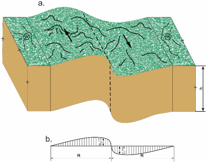
Figure 1. Schematic illustration of a slow and lengthy deformation of the medium over a long period of an earthquake maturing, a. deformed condition of the medium before development of the rupture, b. distribution of displacements of the medium in the direction perpendicular to the rupture before the earthquake, is the depth of the future rupture, is static deformations of blocks the moment rupture occurs, is length of the deformation area perpendicular to the rupture, are regions suggested as not deformed by maturing earthquakes because of relatively small deformations compared to the u at the rupture. Arrows show directions of slow slips of blocks, dashed line shows the line of future rupture.
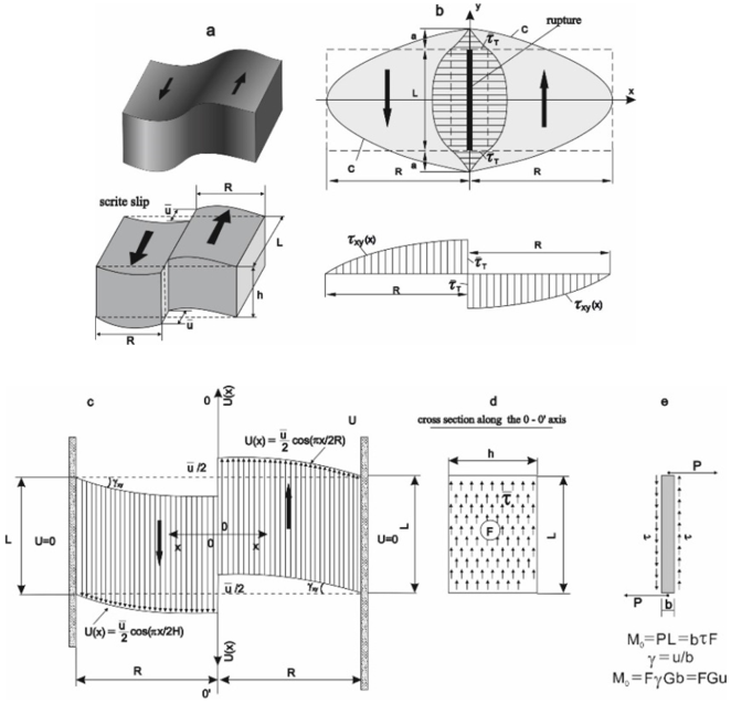
Figure 2. Schematic illustration of the medium stress condition a-before formation of the rupture, b-after formation of the rupture, c-equivalent areas of stress conditions, d-distribution of shear stresses, (<i></i>lim -limit resistance of rocks), e-interpretation of the physical essence of the seismic moment.
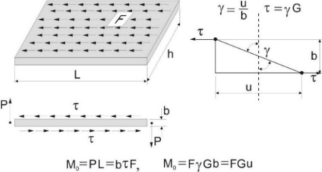
Figure 3. The mechanism of the rupturing process and illustration of the seismic moment’s occurrence [5, 6].
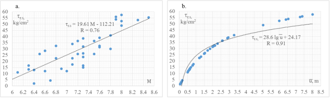
Figure 4. Dependence of stress relief values on: (a) magnitude M, and (b) on mean slip .
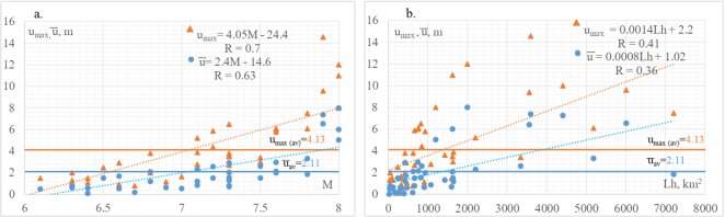
Figure 5. Dependence of maximum slip and mean slip values on: (a) earthquake magnitude , and (b) on rupture area .
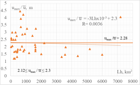
Figure 6. The dependence of the ratio on the rupture area .
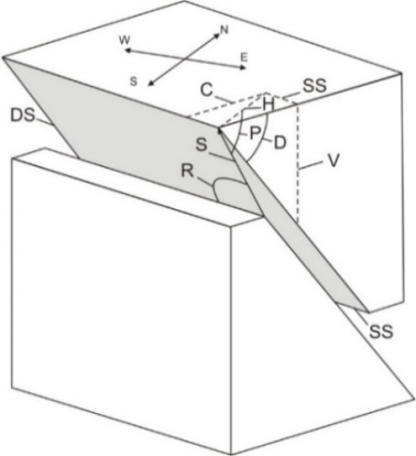
Figure 7. The diagram of surface rupture formation during the Spitak earthquake [15].
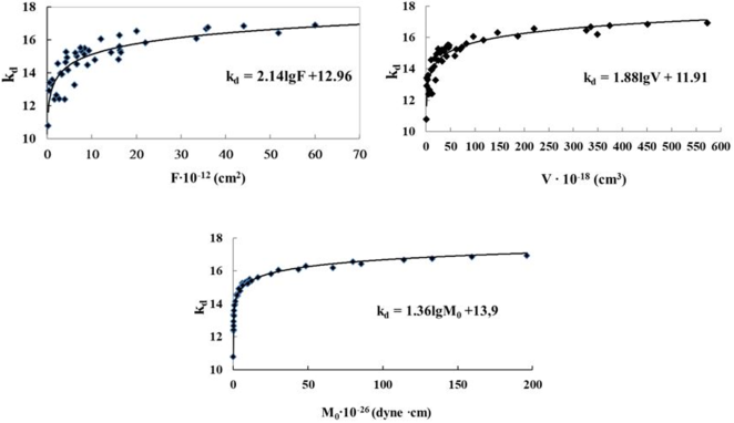
Figure 8. Dependence of the deformation energy class value ![]() , for 44 strong earthquakes with the magnitude on the rupture area , deformation volume and earthquake’s seismic moment .
, for 44 strong earthquakes with the magnitude on the rupture area , deformation volume and earthquake’s seismic moment .
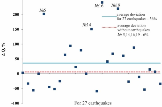
Figure 9. Dependence of aftershock location area differences in percent between formula (16) and empirical formula (15) for 27 earthquakes with magnitudes .
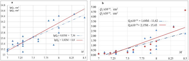
Figure 10. Logarithmic and linear dependencies of aftershock location areas on earthquake magnitude M, based on formulas (15) and (16).
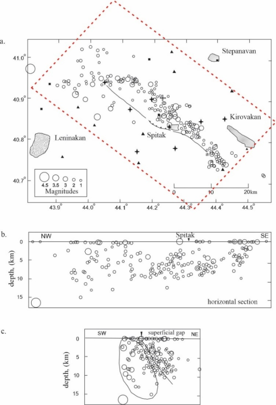
Figure 11. Locations of aftershock epicenters of Spitak earthquake 7.12.1988 [9] and the nominal rectangle (dotted) of calculated aftershocks area. a. geographic location of epicenters b. Projection of hypocenters on the plane of the rupture, c. hypocenters in the zone of the plane perpendicular to the surface [9].
Information


 x 104
x 104 from formula (