Bed Roughness Incorporated Lift Force Formulation for Sediment Concentration Solutions

Tarek Taha

doi:doi:10.11648/j.ajwse.20241001.12

Research Article |

| Peer-Reviewed

Bed Roughness Incorporated Lift Force Formulation for Sediment Concentration Solutions

Tarek Taha^*

Published in American Journal of Water Science and Engineering (Volume 10, Issue 1)

Received: 23 May 2024 Accepted: 11 June 2024 Published: 6 August 2024

Views: Downloads:

Download PDF

Share This Article

Twitter
Linked In
Facebook

Abstract

Within the field of sediment transport dynamics, there is an emphasis on the need for providing and improving simplified analytical solutions from which the findings can be extended upon. Typically, solutions have been developed from the understanding and incorporation of vertical velocity components/distribution; however, there remains opportunity for analytical enhancement. Under uniform open channel dilute sediment laden flow conditions, the type II concentration profile reflects the maximum concentration at a distance from the bed. To analytically depict the type II profile, it is essential to describe the vertical velocity components acting within the flow hydrodynamics. Yet, the impact of bed roughness on the vertical velocity distribution influencing a sediment particle has not been articulated. Hence, in this research, the impact of bed roughness is incorporated into the vertical velocity distribution to formulate the lift force acting upon a particle, to provide a sediment concentration solution. The proposed analytical vertical velocity distribution solution is validated against existing formulations, followed by the proposed sediment concentration being validated against existing solutions. Here, the results indicate that analytically incorporating the bed roughness alongside the secondary current induced vortices provides a lift force solution that can depict the type II concentration profile. Under relatively low shear velocity, increasing the sediment diameter allows for a clearer depiction of the near surface region and profile curvature. Furthermore, the proposed sediment concentration solution can accurately depict the near surface region, curvature of concentration, and maximum concentration under relatively large shear velocity data. Importantly, under conditions where both the shear velocity and sediment diameter are relatively large, the maximum concentration is captured with greater accuracy; however, the curvature of the profile and the near surface region accuracy are hindered. It is to be noted, that due to the formulation of the proposed velocity distribution the accuracy of the solution towards the bed decreases due to instability caused as the characteristic depth decreases to zero.

Published in	American Journal of Water Science and Engineering (Volume 10, Issue 1)
DOI	10.11648/j.ajwse.20241001.12
Page(s)	8-26
Creative Commons	This is an Open Access article, distributed under the terms of the Creative Commons Attribution 4.0 International License (http://creativecommons.org/licenses/by/4.0/), which permits unrestricted use, distribution and reproduction in any medium or format, provided the original work is properly cited.
Copyright	Copyright © The Author(s), 2024. Published by Science Publishing Group

Keywords

Lift Force, Vertical Velocity Components, Vertical Velocity Distribution, Bed Roughness, Sediment Concentration, Type II Profile, Open Channel, Hydrodynamic Solution

1. Introduction

Under open channel conditions, sediments can be transported under two regimes, namely, bed load and suspended load. Bed load transport revolves around sediments travelling along the bed by bouncing, sliding, or rolling. Sediments that undergo bed load transport are generally heavier than sediments undergoing suspended transport and are influenced predominantly by flow velocity, shape and size of sediment. On the other hand, relatively lighter sediment particles will be transported via suspension through the water column, and are influenced primarily by flow turbulence, density, and size of the particles.

It is important to distinguish between the nature of suspended sediment concentrations, which can be categorized as dilute (type I and type II profiles) and hyper-concentrated. Reflected by figure 4, type I concentration profiles refer to a maximum concentration located within the near bed region, where-as type II concentration profiles reflect a maximum concentration at a distance from the channel bottom

[9, 23]

. Both type I and type II concentrations fall within the concentration required to project suspended sediments (critical concentration); however, hyper concentrated concentrations exceed the critical concentration level and can influence the flow to behave uniquely. Naturally, turbulent flows express fluctuations in properties (i.e. velocity and pressure) due to complex dynamics, where the variability of turbulent flow dynamics is captured by dilute and hyper concentrated regimes reflecting the non-linear characteristics of the turbulent regime. Both concentration profiles provide substantial practical application by providing insight on the flow transport mechanism. The realistic conditions expressed by dilute type II and hyper concentrated profiles are attributed to their incorporation of the fluid-particle interactions reflected within the flow regime. Type II concentration profiles are utilised for flow conditions where the fluid-particle interactions are weak, while that of hyper concentrated profiles are used to reflect relatively strong fluid-particle interactions.

Download: Download full-size image

Figure 1. Type I and Type II Suspended Sediment Concentration Profile

[9]

Under dilute concentration conditions, it is assumed that particle-particle interactions are not permanent and do not occur frequently, hence the prominent influencing factors of the dilute profiles are of external forces exhibited within the flow regime

[10]

. This assumption cannot be utilized under hyper concentrated concentrations as particle-particle interactions are deemed permanent and frequent. The permanent and frequent assumptions of particle interactions under hyper concentrated flows complicate the quantification of the sediment concentration, making it difficult to provide simplified solutions under dam break events. Additionally, a substantial modelling consequence of hyper concentrated flows is the dampening effect/nullification of vertical velocity components, such as lift force, which are significant type II external forces

[10]

. Prominent analytical, experimental, and numerical research have demonstrated the significance of vertical velocity components for their influence over the concentration and distribution with the most accurate modelling sediment concentration solutions accounting for both drift and lift force acting upon a sediment

[10]

The lift force is a critical vertical velocity component involved within the dynamics of sediment concentrations, dictating the concentration profile expressed within dilute flow regimes

[10, 18, 24]

. From the literature, the velocity distribution has been a vital essence for analytical development of the lift force, with one of the most relatively recent contributions incorporated the impact of the secondary vortices induced current within the lift force velocity distribution

[9, 10]

. Notably, the lift force velocity distribution lacks consideration for the impact of the bed roughness on the lift force, even though the bed roughness has an impact on the flow depth, energy dissipation, free surface profile, and sediment transport. Hence, the purpose of this research is to produce a sediment concentration solution accounting for the impact of bed roughness upon the lift force dynamics through the vertical velocity distribution. Here, the research novelty contributes to the hydrodynamic field through analytical formulation of vertical velocity components critical to the type II concentration profile, to depict the impact of turbulence structures on the sediment transport mechanism

[24]

2. Literature Review

Sediment concentration solutions based on 3D governing equations consider the three spatial dimensions, providing the greatest level of detail regarding the sediment-flow dynamics. However, 3D solutions are naturally complex and will require significant number of data inputs and computational demand while experiencing a sensitivity to simulation parameters such as settling velocity. Additionally, obtaining accurate values for 3D solutions is troublesome as many parameters vary spatially and temporally, with other parameters also requiring field measurement or calibration. On the other hand, 2D governing equations exhibit characteristics of simplicity and comprehensive ability with respect to 3D and 1D solutions. Sediment concentration solutions based on 2D governing equations can capture complex sediment-fluid dynamics such as lift force acting on a particle due to the contribution of both fluid shear and particle rotation, while offering manageable complexity in solution representation.

2.1. Governing Equations

Sediment concentration solutions can be 2D single phase, or 2D two phase based, where the main concern of using a single fluid-based solution is that the effects of sediment particles on turbulent structures are not considered. For instance, diffusion theory physically revolves around implicating only, gravitational forces, vertical drag, and buoyancy effects in-which they are considered, whereas particle inertia, fluid-particle interactions and particle-particle interactions are not considered. For single phase models, research conducted on sediment concentrations can be based upon the kinetic theory of granular flow or the probability density function (PDF). On the other hand, two phase liquid-solid solutions describe a methodology that accounts for both flow and the sediments within the water body.

Two phase solid liquid solutions consider solid particle cloud and ambient fluid as continuous media, if the sizes of the solid particles are significantly smaller than the macro geometric dimension of the flow considered

[24]

. This condition is well satisfied in sediment laden flows commonly encountered in fluvial rivers and manmade channels where suspended sediment transport is predominant. Two phase models can be presented to resemble the Rouse model (classic diffusion convection) to simulate the vertical direction where the gradient of turbulence is influenced by the concentration gradient generating a drift flow

[8]

. However, the two-phase solution method has been criticized predominantly due to the continuum theory being insufficient in describing the solid-particles relationship, which for sediment concentration solutions this drawback is significant. To overcome this, it is of substantial importance that the kinetic theory is incorporated

[10]

. The kinetic theory originates from the kinetic theory of gases, and assumes that matter is composed of numerous molecules, and that these molecules are in constant state of ceaseless motion.

Assumptions of the kinetic theory are (i) molecules interact with each other, (ii) macroscopic state and qualities of matter are derived through the synthesis of molecular behaviour and (iii) particles are of equivalent shape but of different radius

[10, 24]

. The solution method of kinetic two-phase flows comprises four main steps: (i) to establish governing equations, (ii) establish forces acting upon particles, (iii) substituting into the governing equations followed by (iv) the implementation of closure equations and dimensionless formulation. To account for the stresses generated by the sediment particles at the surface, and to maintain the consistency with two phase models and kinetic theory of granular flows, many prominent studies assume the surface of the control volume to be one with the fluid phase and interact with the present sediments, an assumption only valid under conditions of temporary particle-particle interactions

[10, 24]

The two-phase kinetic theory can be based on the Boltzmann equation of velocity distribution, where the sediment particles and fluid comprise drag, lift, virtual mass and Basset History force

[11]

. For a 2D incompressible fully turbulent dilute sediment-laden flow evaluation following the momentum equilibrium of group particle motion under uniform channel slope conditions, the conservation of mass and momentum can be reflected as

\frac{\partial C}{\partial t} + \frac{\partial}{\partial x} (C u_{s}) + \frac{\partial}{\partial d_{z}} (C v_{s}) = 0

(1)

C [\frac{\partial v_{s}}{\partial t} + u_{s} \frac{\partial v_{s}}{\partial x} + v_{s} \frac{\partial v_{s}}{\partial d_{z}}] = C g_{z} - \frac{C}{ρ_{s}} \frac{\partial p}{\partial d_{z}} + \frac{1}{ρ_{s}} \frac{\partial σ_{s}}{\partial d_{z}} + \frac{1}{ρ_{s}} F_{sz}

(2)

Here, ‘C’ is the volume fraction of sediment particles of uniform rounded sediment particle diameter, ‘t’ reflects dimensionless time, ‘x’ and ‘

d_{z}

’ represent the longitudinal and vertical dimensions, ‘

u_{s}

’ and ‘

v_{s}

’ annotate the instantaneous particle velocity components in respect to ‘x’ and ‘

d_{z}

’, ‘

g_{z}

’ is the the component of gravity acceleration in respect to ‘

d_{z}

’, ‘

ρ_{s}

’ reflects the sediment density, ‘p’ annotates water pressure, ‘

σ_{s}

’ reflects the particle-particle interactions generated stress and the phase interaction forces are annotated by ‘

F_{sz}

’. Under the assumption of under uniform channel slope conditions, resolving ‘

g_{z}

’ horizontally gives,

g_{z} = - gcosθ \approx - g

The theory of 2D kinetic two-phase conservation of mass and momentum treats the sediment particles and the body of water as two separate mass points with two different densities; eliminating the inertia terms from both fluid and sediment particle representation, reflecting the sediment concentration only from the vertical direction. From this, combining equations (1) and (2) provides the governing equations of the vertical distribution of sediment particles under open channel flow conditions

[7, 10]

(C v_{s}) \frac{\partial}{\partial t} + (C u_{s} v_{s}) \frac{\partial}{\partial x} + (C v_{s} v_{s}) \frac{\partial}{\partial d_{z}} = - Cg - \frac{C}{ρ_{s}} \frac{\partial ρ}{\partial d_{z}} + \frac{1}{ρ_{s}} \frac{\partial σ_{s}}{\partial d_{z}} + \frac{1}{ρ_{s}} F_{sz}

(3)

A linear variation of shear stress over the flow depth is to be assumed, however, this has been debated, noting that the velocity distribution is not linear across the flow depth

[20, 21]

. Expressing the Reynolds decomposition to the instantaneous velocities ‘

u_{s} = \overset{̅}{u_{s}} + u_{s}^{'}

’ and ‘

v_{s} = \overset{̅}{v_{s}} + v_{s}^{'}

’, where ‘

\overset{̅}{u_{s}}

’ and ‘

\overset{̅}{v_{s}}

’ represent the respective time average component and the fluctuation component is noted by ‘

u_{s}^{'}

’ and ‘

v_{s}^{'}

’ and time averaging equations (3) provides

[11, 24]

\overset{̅}{v_{s}} [\frac{\partial \overset{̅}{C}}{\partial t} + \frac{\partial}{\partial x} (\overset{̅}{C u_{s}} + \overset{̅}{C' u_{s}^{'}}) + \frac{\partial}{\partial d_{z}} (\overset{̅}{C v_{s}} + \overset{̅}{C' v_{s}^{'}})] + \overset{̅}{C} \frac{\partial \overset{̅}{v_{s}}}{\partial t} + (\overset{̅}{C u_{s}} + \overset{̅}{C' u_{s}^{'}}) \frac{\partial \overset{̅}{v_{s}}}{\partial x} + (\overset{̅}{C v_{s}} + \overset{̅}{C' v_{s}^{'}}) \frac{\partial \overset{̅}{v_{s}}}{\partial d_{z}} + \frac{\partial \overset{̅}{C' v_{s}^{'}}}{\partial t}

+ \frac{\partial}{\partial x} (\overset{̅}{C u_{s}^{'} v_{s}^{'}} + \overset{̅}{C {u_{s} v}_{s}^{'}} + \overset{̅}{C' u_{s}^{'} v_{s}^{'}}) + \frac{\partial}{\partial d_{z}} (\overset{̅}{C v_{s}^{'} v_{s}^{'}} + \overset{̅}{C {v_{s} v}_{s}^{'}} + \overset{̅}{C' v_{s}^{'} v_{s}^{'}}) =

- \overset{̅}{C} g - \frac{\overset{̅}{C}}{ρ_{s}} \frac{\partial \overset{̅}{p}}{\partial d_{z}} - \frac{1}{ρ_{s}} \overset{̅}{C^{'} \frac{\partial p^{'}}{\partial d_{z}}} + \frac{1}{ρ_{s}} \frac{\partial \overset{̅}{σ_{s}}}{\partial d_{z}} + \frac{1}{ρ_{s}} \frac{\partial \overset{̅}{R_{s}}}{\partial d_{z}} + \frac{1}{ρ_{s}} {\overset{̅}{F}}_{sz}

(4)

Where, average components are reflected by

\overset{̅}{overbars}

and the fluctuating components are reflected by

{primes}^{'}

the average Reynolds shear stress generated by velocity fluctuations is reflected as ‘

\overset{̅}{R_{s}} = - ρ_{s} \overset{̅}{v_{s}^{'} v_{s}^{'}}

’. Under steady non uniform open channel flow it can be assumed that rates of change in respect to the longitudinal dimension (

\frac{\partial}{\partial x})

and time (

\frac{\partial}{\partial t})

are zero, hence combing equations (1) and (4) provides,

(\overset{̅}{C v_{s}} + \overset{̅}{C' v_{s}^{'}}) \frac{\partial \overset{̅}{v_{s}}}{\partial d_{z}} + \frac{\partial}{\partial z} (\overset{̅}{C v_{s}^{'} v_{s}^{'}} + \overset{̅}{C {v_{s} v}_{s}^{'}} + \overset{̅}{C' v_{s}^{'} v_{s}^{'}}) = - \overset{̅}{C} g - \frac{\overset{̅}{C}}{ρ_{s}} \frac{\partial \overset{̅}{p}}{\partial d_{z}} - \frac{1}{ρ_{s}} \overset{̅}{C^{'} \frac{\partial p^{'}}{\partial d_{z}}} + \frac{1}{ρ_{s}} \frac{\partial \overset{̅}{σ_{s}}}{\partial d_{z}} + \frac{1}{ρ_{s}} \frac{\partial \overset{̅}{R_{s}}}{\partial d_{z}} + \frac{1}{ρ_{s}} {\overset{̅}{F}}_{sz}

(5)

Time averaging the conservation of mass equation for steady uniform flow implies ‘

\frac{\partial}{\partial d_{z}} (\overset{̅}{C v_{s}} + \overset{̅}{C' v_{s}^{'}})

’ is zero, and under equilibrium sediment transport the net mass flux ‘

\overset{̅}{C v_{s}} + \overset{̅}{C' v_{s}^{'}}

’ is also zero. From this equation (5) can be represented as,

\frac{\partial}{\partial z} (\overset{̅}{C v_{s}^{'} v_{s}^{'}} + \overset{̅}{C {v_{s} v}_{s}^{'}} + \overset{̅}{C' v_{s}^{'} v_{s}^{'}}) = - \overset{̅}{C} g - \frac{\overset{̅}{C}}{ρ_{s}} \frac{\partial \overset{̅}{p}}{\partial d_{z}} - \frac{1}{ρ_{s}} \overset{̅}{C^{'} \frac{\partial p^{'}}{\partial d_{z}}} + \frac{1}{ρ_{s}} \frac{\partial \overset{̅}{σ_{s}}}{\partial d_{z}} + \frac{1}{ρ_{s}} \frac{\partial \overset{̅}{R_{s}}}{\partial d_{z}} + \frac{1}{ρ_{s}} {\overset{̅}{F}}_{sz}

(6)

The turbulent diffusion velocity of sediment particles (

U_{s}^{T}

) can be used to transform ‘

\overset{̅}{C {v_{s} v}_{s}^{'}}

’ into ‘

\overset{̅}{C v_{s}} U_{s}^{T}

’, where ‘

T

’ reflects the period taken in which the time average of fluctuating velocity (

\overset{̅}{u_{s}^{'}}

) becomes zero. However, the turbulent diffusion velocity of sediment particles (

U_{s}^{T}

) is insignificant, hence the ‘

\overset{̅}{C v_{s}} U_{s}^{T}

’ term can be neglected; alongside the higher order correlation (

\overset{̅}{C' v_{s}^{'} v_{s}^{'}}

) term due to the complex expressions of the resultant equations

[10, 12]

Pressure fluctuations of turbulent flows are generated by turbulence intensities, where the particle Reynolds number ‘

{Re}_{p}

’ determines the weaking or strengthening of the flow turbulence intensities. Under the dilute flow conditions, for type II concentrations the trailing vortices will not detach from particles due to the turbulence intensities not to increase allowing for the pressure fluctuation term to be eliminated

[10]

. Hence, the governing equation for sediment transport under steady uniform open channel is,

\frac{\partial}{\partial z} (C v_{s}^{' 2}) = - Cg (1 - \frac{ρ_{f}}{ρ_{s}}) + \frac{1}{ρ_{s}} \frac{\partial R_{s}}{\partial d_{z}} + \frac{1}{ρ_{s}} \frac{\partial σ_{s}}{\partial z} + \frac{1}{ρ_{s}} F_{sz}

(7)

Here, ‘

\frac{ρ_{f}}{ρ_{s}} = \frac{\partial p}{\partial z}

’ where ‘

ρ_{f}

’ reflects the density of the fluid phase, ‘

(C v_{s}^{' 2}) \frac{\partial}{\partial z}

’ is the rate of momentum transport by sediment particle fluctuations, ‘

- Cg (1 - \frac{ρ_{f}}{ρ_{s}})

’ represent the gravity on particles in a body of water. To continue, the vertical particle forces ‘

F_{sz}

’ must be formulated.

The turbulence fluid sediment correlations follow that of the fluid phase turbulence

[5]

; however, this is criticized due to sediment particles not instantaneously responding to changes in the flow velocity, and that the mean fluid velocity is larger than that of the mean sediment velocity

[10]

. In addition to this, relatively large particles will require a longer time to respond to the forces expressed by the fluid in respect to relatively small particles. To address this, many studies have assumed a uniform sediment diameter per simulation

[10, 17, 24]

, allowing for the turbulence intensity of particles to be proportional to the turbulence intensity of fluid; however, such a methodology will still overestimate concentration levels due to the formulation of sediments reacting instantaneously to the flow intensities

[9, 10]

Some studies adopted a solid-liquid two phase solution where the turbulence intensity of the solid phase is assumed constant, and the turbulence intensity lift force is neglected

[24]

. However, these assumptions restrict the solution from presenting a detailed variation of concentration profile towards/at the near bed region (NBR). Under the assumption that the turbulence intensity of particles is proportional to the turbulence intensity of the fluid the NBR can be depicted with more accuracy, assumed that due to the centrifugal forces generated by the sediment particles being affected by the turbulence eddies, the dispersion increases

[5, 7, 10]

. However, due to the sediments within the flow, the fluid turbulence intensities are damped in the NBR, whereas at a distance from the bed where sediment concentration is considerably less, the turbulence intensity of the fluid is much greater and can overcome the damping effect of the sediment particles

[7]

2.2. Vertical Forces Acting on a Particle

To describe the (vertical) forces acting on a particle, the external forces, incorporated into two phase sediment concentration solutions differ in representation, with general considerations being drag, added mass and lift force

[5, 7]

. The drag and lift force are prominent turbulence structures reflected by ejection and sweep burst cycle events, highlighting the significance of the external forces in relation to vertical velocity components. Importantly, the vertical velocity components influence the sediment concentrations along the vertical direction, emphasising the importance of the lift force

[1, 10]

. Additionally, the literature notes that the lift force has substantial impact on dilute concentration distribution, noting its importance in reflecting type II sediment concentrations in the near bed region

[10, 17, 24]

. This is because, within the near bed region, the velocity fluctuations contribute to the gravitational settlement of sediments and a major advantage of kinetic theory solutions is in their inclusion of sediment lift force and velocity fluctuations alongside drag force

[10]

Studies have accounted for the lift force ‘

F_{L}

’ as all the vertical forces acting on a sediment excluding drag force

[10, 24]

. This research considers all the resultant forces acting on a particle excluding drag force ‘

F_{D}

’ to be denoted as the time averaged force ‘

M_{sz}

’

[10]

. Therefore, the forces acting on a particle ‘

F_{sz}

’can be reflected as,

F_{sy} = F_{D} {+ M}_{sz}

(8)

The drag and lift force (vertical velocity components) are the most potent of the external forces, due to the directly proportionate relationship with the distribution of suspended sediment concentration near the bed region

[6, 13]

. Under uniform sediment diameter, the drag force acting on a sediment travelling vertically can be reflected as

[10]

F_{D} = {\frac{1}{2} ρ}_{f} C_{D} (\frac{π d^{2}}{4}) v_{r}^{2}

(9)

Here, ‘

C_{D}

’ is the coefficient of drag and the relative velocity of a particle to the fluid is denoted by ‘

v_{r}^{2} = v_{s} - v_{f}

’, where ‘

v_{f}

’ reflects the vertical velocity of the fluid phase. The instantaneous vertical velocity of the solid phase ‘

v_{s} = v_{f} - ω_{0}

’ where ‘

ω_{0}

’ reflects the sediment settling velocity. From this, the drift force of rounded sediments of constant diameter can be derived as,

F_{D} = {\frac{1}{2} ρ}_{f} C_{D} (\frac{π d^{2}}{4}) ω_{0}^{2}

(10)

The drag force coefficient ‘

C_{D}

’ is a function of the particle Reynolds number, and that a particle experiences both laminar flow and turbulent flow during its suspension. For Stokes flow ‘

{Re}_{p} < 1

’, flow around sphere is laminar and drag coefficient follows the linear relation ‘

C_{D} = \frac{24}{{Re}_{p}}

’. Additionally, when ‘

{Re}_{p} < 10^{5}

’, the drag force coefficient ‘

C_{D} \approx 0.5

’. Where, ‘

Φ

’ is a function of the particle Reynolds number (

{Re}_{p}

) and ‘

Φ \approx 0

’ when ‘

{Re}_{p} < 1

’

[10].

Hence the drag coefficient can be reflected as,

C_{D} = \frac{24}{{Re}_{p}} + Φ ({Re}_{p})

(11)

Substituting the drag coefficient (equation 11) into the drag force equation (equation 10) provides,

F_{D} = {\frac{π d^{2}}{8} ρ}_{f} \frac{24}{{Re}_{p}} ω_{0}^{2} + {\frac{π d^{2}}{8} ρ}_{f} Φ ({Re}_{p}) ω_{0}^{2}

(12)

Here, the ‘

{\frac{π d^{2}}{8} ρ}_{f} \frac{24}{{Re}_{p}} ω_{0}^{2}

’ term denotes the particle Stokes drag force under laminar flow and the ‘

{\frac{π d^{2}}{8} ρ}_{f} Φ ({Re}_{p}) ω_{0}^{2}

’ term denotes the effect of particle fluctuation.

Various studies have accounted for the nonlinear dependence of drag force on the particle slip Reynolds number through the drag force representation but eliminated the drift velocity

[3, 21, 22, 24]

. However, the drift force must incorporate drift velocity as when a particle moves through turbulent flow due to velocity fluctuation and correlation between instantaneous particle distribution, random fluctuations are generated and consequently a diffusive flux is created affecting the movement of particles through drift velocity

[7, 16]

. To account for this, the time averaged drag force can be decomposed into two parts, under the assumption that fluid in close approximation to particles will be of a laminar nature, and as the distance increases from the particle, the flow expresses a turbulent nature. From this, the drag force can be reflected as (i) a linear coupling of laminar drag force and (ii) the influence of particle fluctuations due to flow turbulence and collision

[9, 10]

F_{D} = F_{DL} {+ F}_{DT}

(13)

Here, the laminar drag force component is reflected as ‘

F_{DL}

’, and the turbulent drag force component is reflected as ‘

F_{DT}

’. During the descent of a sediment due to gravity, the laminar drag force is equal to that of the submerged weight of the sediment, referred to as buoyancy force. From this, the laminar drag force (

F_{DL}

) can be reflected as

[10]

F_{DL} = C ρ_{s} g (1 - \frac{ρ_{f}}{ρ_{s}})

(14)

The time-averaged turbulent drag force and the ratio of difference of drift velocities of two phases are proportional to each other, in respect to the integral turbulence timescale. Where the ratio of the relative particle velocity to a particle timescale is ‘

τ_{p}

’. From this, the turbulent drag force ‘

F_{DT}

’ is represented as

[10]

F_{DT} = C ρ_{s} (S t_{b} - 1) \frac{ω_{o}}{τ_{p}}

(15)

Hence, the final equation representing the drag force on a particle is,

F_{D} = C ρ_{s} g (1 - \frac{ρ_{f}}{ρ_{s}}) + C ρ_{s} (S t_{b} - 1) \frac{ω_{o}}{τ_{p}}

(16)

Here, drag force is considered to account for velocity relative of the particle to the fluid, and the vertical velocity of the fluid phase. Where the vertical velocity of sediment particles is the addition of vertical velocity of fluid and the sediment settling velocity. On the other hand, the lift force accounts for all external forces excluding drag and can be expressed as a time averaged force. In part, this is due to the behaviour of dilute sediments, which are prone to lift if they are larger in size than the thickness of the viscous sub-layer otherwise the sediments stay within the bed layer

[6]

. Similar to the drag force, the lift force representation varies across studies

[10, 17, 24]

. From the literature, fluid lift force is generated through (i) the movement of sediment from the fluid shear due to flow velocity gradient, and/or (ii) the rotation of sediments. It is assumed that the lift force acting on a particle is due to the contribution of both fluid shear and particle rotation. From this the time averaged force is represented as

[9]

M_{sz} = C ρ_{s} L_{y}

(17)

Here, ‘

L_{y}

’ denotes lift force per unit mass on particle, which is derived from the lift force ‘

F_{L}

’, reflected as the resultant force of all other external force excluding drag force through the fluid shear and particle orientation assumption,

L_{y} = \frac{6 F_{L}}{π ρ_{s} d^{3}}

(18)

the lift force (

F_{L}

) is derived as

[1, 10]

F_{L} = \frac{4 π}{3} C_{L} ρ_{f} d^{3} u_{r} \frac{\partial u_{f}}{\partial d_{z}}

(19)

Here ‘

C_{L}

’ reflects the coefficient of lift, ‘d’ represents sediment diameter, ‘

u_{r}

’ illustrates the relative velocity of sediments in respect to the fluid, ‘

u_{f}

’ is the velocity of the fluid phase along the streamwise direction. The relative velocity of sediments in respect to the fluid is reflected as ‘

u_{r} = u_{f} - u_{s} + u_{d}

’, where ‘

u_{s}

’ is the mean velocity of sediments along the stream wise direction and ‘

u_{d}

’ is the drift velocity

[9, 10]

. The drift velocity is usually ignored

[13]

, however, due to the correlation between the fluid velocity fluctuations and the instantaneous sediment distribution, the drift velocity should be accounted for as

[10]

u_{d} = - D (\frac{1}{C} \frac{\partial C}{\partial d_{z}} - \frac{1}{1 - C} \frac{\partial (1 - C)}{\partial d_{z}})

(20)

Here, the drift diffusion is reflected as ‘

D = {- τ}_{t} \overset{̅}{v_{f}^{'} v_{s}^{'}} = - \frac{τ_{p}}{{St}_{b} - 1} \overset{̅}{v_{f}^{'} v_{s}^{'}}

’ where ‘

τ_{t}

’ is the net drag force due to turbulent motion. During the propagation of sediments, a velocity lag between the fluid phase and sediment phase is experienced, influencing the flow depth. The lag velocity is denoted by ‘

u_{l} = u_{f} - u_{s}

’, and hence can be derived as

[10]

u_{l}^{+} = \frac{u_{l}}{u_{*}} {[\sqrt{(2 - 2 \frac{z}{h})^{\frac{1}{1.5}} + \frac{1}{4} (32 \frac{v_{fk}}{u_{*} d})^{\frac{2}{1.5}}} - \frac{1}{2} (32 \frac{v_{fk}}{u_{*} d})^{\frac{1}{1.5}}]}^{1.5}

(21)

Here, (

v_{fk})

reflects the kinematic viscosity of the fluid, from this the relative velocity (

u_{r}

) can be derived as,

\frac{u_{r}}{u_{*}} = \frac{u_{l}}{u_{*}} + \frac{(\frac{ω_{o}}{u_{*}}) \overset{̅}{v_{fk}^{'} v_{s}^{'}}}{gC (1 - C) (S_{tb} - 1) (1 - \frac{ρ_{f}}{ρ_{s}})} \frac{\partial C}{\partial d_{z}}

(22)

The velocity distribution can be incorporated into the lift force as

[10]

\frac{u_{f}}{u_{*}} = \frac{1}{k} \ln \frac{y}{h} + B_{r} + \frac{2 Π}{k} si n^{2} (\frac{πy}{2 h})

(23)

The ‘

\frac{1}{k} \ln \frac{y}{h}

’ term represents the logarithmic function of which ‘k’ represents the dimension-less constant utilized in logarithmic law to reflect the distribution of logarithmic velocity. The ‘

\frac{2 Π}{k} si n^{2} (\frac{πy}{2 h})

’ term possesses similarities to that of Jasmund-Nikuradse logarithmic velocity profile

[15]

. The second term, ‘B_r’, is the logarithmic integration constant. From this the lift force per unit mass can be derived by incorporating the effect of secondary vortices induced current within the velocity distribution

[10]

. Once again highlighting the potent relationship between vertical velocity component (lift force), turbulence (generated by the secondary vortices induced current) and the sediment concentration. Under the assumption that the flow propagates in the streamwise direction and due to the transverse flow effects, ridges and troughs are generated parallel to the longitudinal flow direction in an alternative manner. Alongside the assumption that secondary cells are symmetrical in respect to their circulation center, the rotation of the vortex naturally generates and influences vertical forces tangentially. The rotational force is assumed to be equal at the tangent-circumference location. These tangent locations on the circumference of the circular motion can be illustrated as function of vertical-characteristic length ‘

si n^{2} (\frac{πy}{2 h}) \approx si n^{2} \frac{π ξ_{n}}{2}

’. Hence the lift force can be reflected as

[10]

L_{y} = λ_{2} \frac{u_{*}^{2}}{h} [\frac{1}{ξ_{n}} + 12 Π (ξ_{n}) (1 - ξ_{n})] [\frac{u_{l}}{u_{*}} + \frac{ϕ}{C (1 - C)} \frac{\partial C}{\partial d_{z}}]

(24)

Hence time averaged force (

M_{sz}

) can be represented as,

M_{sz} = C ρ_{s} λ_{2} \frac{u_{*}^{2}}{h} [ξ_{n} + 12 Π (ξ_{n}) (1 - ξ_{n})] [\frac{u_{l}}{u_{*}} + \frac{ϕ}{C (1 - C)} \frac{\partial C}{\partial d_{z}}]

(25)

From this the particle forces (

F_{sz}

) can be evaluated as,

F_{sz} = C ρ_{s} g (1 - \frac{ρ_{f}}{ρ_{s}}) + C ρ_{s} (S t_{b} - 1) \frac{ω_{o}}{τ_{p}} + C ρ_{s} λ_{2} \frac{u_{*}^{2}}{h} [\frac{1}{ξ_{n}} + 12 Π (ξ_{n}) (1 - ξ_{n})] [\frac{u_{l}}{u_{*}} + \frac{ϕ}{C (1 - C)} \frac{\partial C}{\partial d_{z}}]

(26)

The particle forces (

F_{sz}

) can be substituted into the dynamic wave equation (momentum equation),

C \frac{\partial \overset{̅}{v_{s}^{' 2}}}{\partial d_{z}} + \overset{̅}{v_{s}^{' 2}} \frac{\partial C}{\partial d_{z}} = C (S t_{b} - 1) \frac{ω_{o}}{τ_{p}} + λ_{2} C (\frac{u_{*}^{2}}{h}) [\frac{1}{ξ_{n}} + 12 Π (ξ_{n}) (1 - ξ_{n})] [\frac{u_{l}}{u_{*}} + \frac{ϕ}{C (1 - C)} \frac{\partial c}{\partial d_{z}}] + \frac{1}{ρ_{s}} \frac{\partial R_{s}}{\partial z} + \frac{1}{ρ_{s}} \frac{\partial σ_{s}}{\partial z}

(27)

From the literature, the sediment coefficient can be reflected as ‘

ε_{s} = τ_{p} \overset{̅}{v_{s}^{' 2}}

’ and the Stokes bulk number as ‘

S t_{b} = \frac{τ_{p} u_{*}}{h}

’ and through normalizing the sediment coefficient, sediment settling velocity, turbulence intensity of solid phase, the particle stress, lag velocity, and the Reynolds shear stress generated due to sediment velocity fluctuations, equation (27) can be reflected as

[10, 24]

[ε_{s}^{+} - \frac{λ_{2} S_{tb} Ψ (ξ_{n}) ϕ^{+}}{1 - C}] \frac{\partial C}{\partial ξ} = C ω_{0}^{+} (S_{tb} - 1) + S_{tb} [λ_{2} C Ψ (ξ_{n}) u_{l}^{+} - \frac{C \partial v_{s}^{+ 2}}{\partial ξ_{n}} + \frac{\partial σ_{s}^{+}}{\partial ξ_{n}} + \frac{\partial R_{s}^{+ 2}}{\partial ξ_{n}}]

(28)

Here, the functions ‘

Ψ (ξ_{n}) =

[\frac{1}{ξ_{n}} + 12 Π (ξ_{n}) (1 - ξ_{n})]

’ and ‘

ϕ^{+} = \frac{ϕ}{h} = \frac{\frac{ω_{0}}{u_{*}}}{gh (S t_{b} - 1) (1 - \frac{ρ_{f}}{ρ_{s}})} \overset{̅}{v_{f}^{'} v_{s}^{'}}

’. Where the ‘

[ε_{s}^{+} - \frac{λ_{2} S_{tb} Ψ (ξ_{n}) ϕ^{+}}{1 - C}] \frac{\partial C}{\partial ξ_{n}}

’ term reflects the diffusion generated from (i) the sediment concentration vertical gradient and (ii) sediment drift velocity while accounting for bed roughness.

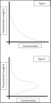
Evidently, the two-phase kinetic theory provides valued and accurate results in presenting the type II sediment concentration solutions due to the inclusion of both drag and lift force acting on a particle as external forces. It is important to note, that when the Stokes number and the lift force coefficient are significantly small, the type I profile (Rouse-type concentration profile) is generated. On the other hand, when the Stokes number is fixed, and the lift force coefficient is increased, the concentration distribution provides a type II profile. This highlights the importance of the lift force on sediment concentration profiles

[10]

The 2D two-phase kinetic theory provides comprehensive detail incorporating vertical velocity components and turbulence dynamics while providing a less demanding and complicated solution in respect to 3D models. The descriptions of the governing equations, fluid drag, and lift force differ across the literature methodologies. However, it is evident key assumptions must be made to present a detailed description of the type II sediment concentration profile, which may limit the comprehensive extension to other research areas, i.e., particle-particle interactions.

From this the vertical velocity can be defined as

[10]

\frac{v}{u_{*}} = αk {ξ_{n}}^{m} (1 - ξ_{n})^{p}

(29)

Here, the characteristic length is reflected as ‘

ξ_{n} = ξ = \frac{d_{z}}{h}

’, and the indices ‘m’ and ‘p’ are dependent on influences of channel geometry obtained from experimental data. The literature reflects the indirectly proportionate behaviour of which the vertical velocity decreases as the values of ‘m’ and ‘p’ increase. The parameter ‘

α

’ may be represented as greater than, equal to, or less than zero, depending on the upward, downward, and parallel to lateral vertical velocity direction

[9]

. Parameter ‘

α

’ is laterally derived as,

α = m_{1} α_{0} η_{*}^{m_{1} - 1} (1 - \frac{m_{1} + 1}{m_{1}} η_{*})

(30)

Where ‘

α_{0}

’ describes the strength of the secondary current, ‘

λ_{1}

’ represents half a width of rough strip, ‘

m_{1} = \frac{λ_{1}}{({λ - λ}_{1})}

’ and ‘

η_{*} = \frac{b - z}{λ}

’. At the middle of the flow depth, the shape of the secondary cells is perceived to be symmetrical in respect to its circulation center where ‘b’ reflects the channel width the vertical velocity can be reflected as

[9]

\frac{v}{u_{*}} = - \frac{v_{\max}}{u_{*}} \sin (π ξ_{n}) \cos (π \frac{b - z}{λ})

(31)

Here, ‘

λ

’ represents the width of the secondary. Substituting equation (30) into equation (31) provides,

\frac{v}{u_{*}} = m_{1} α_{0} k (\frac{b}{2 λ})^{m_{1} - 1} [1 - \frac{m_{1} + 1}{m_{1}} \frac{b}{2 λ}] ξ_{n}^{m} (1 - ξ_{n})^{p}

(32)

Under the approximation of ‘

\sin (π ξ_{n}) \approx 4 ξ (1 - ξ_{n})

’ within the region of ‘

0 \leq π ξ_{n} \leq π

’; the mean vertical velocity can be reflected as

[9]

\frac{v}{u_{*}} \approx - 4 (\frac{v_{\max}}{u_{*}}) \cos (\frac{πb}{2 λ}) ξ_{n} (1 - ξ_{n})

(33)

The sediment concentration flow adheres to the streamwise, simultaneously due to the transverse flow effects, ridges and troughs are generated parallel to the longitudinal flow direction in an alternative manner. Under the assumption that secondary cells are symmetrical in respect to their circulation center. Under this assumption the vertical velocity can be reflected as

[9]

\frac{v}{u_{*}} = - \frac{v_{\max}}{u_{*}} \sin (π ξ_{n}) \cos (π \frac{b - z}{λ})

(34)

The rotation of the vortex naturally generates and influences vertical forces tangentially. The rotational force is assumed to be equal at the tangent-circumference location. These tangent locations on the circumference of the circular motion can be illustrated as function of vertical-characteristic length ‘

si n^{2} \frac{π ξ_{n}}{2}

’.

3. Methodology

3.1. Novel Lift Force Formulation

Originally, Cole’s log-wake law reflects the superposition of the law of the wall due to the wall shear stress and the law of the wake due to the free turbulence at the centreline. The log wake law derived for turbulent boundary layers and pipe flows has since been extended to fit under turbulent open channel flow conditions, reflected as the modified log wake law

[9]

. The modified log wake law consists of two main contributions; the first, is a logarithmic function, a dimensionless constant used in logarithmic law describing the distribution of the longitudinal velocity. The second contribution is an accumulation of two terms, one being Cole’s parameter reflecting a function of the pressure gradient and the other being an additional constant describing the inner region (viscous sublayer and generation layer) of the flow. The modified log wake law describes the velocity distribution and can be extended to incorporate the sediment distribution by incorporating an additional term. Under fully developed turbulent momentum equations, the log wake velocity distribution in sediment laden flows can be reflected as

[10]

\frac{u_{f}}{u_{*}} = \frac{1}{k} \ln \frac{(d_{z} - d_{z 0})}{k_{s}} + B_{r} + \frac{2 Π}{k} si n^{2} (\frac{πz}{2 h})

(35)

Here, the ‘

\frac{1}{k} \ln \frac{(d_{z} - {dz}_{o})}{k_{s}}

’ term represents the logarithmic function of which ‘k’ represents the dimension-less constant utilized in logarithmic law to reflect the distribution of logarithmic velocity. The ‘

\frac{2 Π}{k} si n^{2} (\frac{πz}{2 h})

’ term possesses similarities to that of Jasmund-Nikuradse logarithmic velocity profile. The term ‘

d_{z}

’ reflects the respective depth and ‘

d_{z 0}

’ depicts initial depth. ‘k_s’ represents the Nikuradse roughness coefficient and is dimensionless due to its derivation (

\frac{Ks}{d_{z}}),

and is usually given a value from 1 to 2.5 for immobile beds

[2]

. The second term, ‘B_r’, is the logarithmic integration constant. The shortcoming of the presented modified log wake law is that it deteriorates in validity as the vertical distance approaches zero in the near bed viscous wall region; due to ‘

\ln (\frac{d_{z} - d_{z 0}}{k_{s}})

’ term approaching negative infinity as the vertical distance approaches zero.

The component within the modified log-wake velocity distribution incorporating the effect of secondary current induced vortices is the ‘

\frac{2 Π}{k} (3 ξ_{n}^{2} - 2 ξ_{n}^{3})

’ term; which assumes that ‘

si n^{2} \frac{πξ}{2} \approx (3 ξ_{n}^{2} - 2 ξ_{n}^{3})

’ within the region of ‘

0 \leq π ξ_{n} \leq π

’

[10]

. This is derived from the assumption that at the middle of the flow depth above the interface of rough and smooth strips, the shape of the secondary cells is perceived to be symmetrical in respect to its circulation centre. From this, this research will re-write equation (35) to incorporate the influence of secondary current induced vortices as,

\frac{u}{u_{*}} = \frac{1}{k} \ln (\frac{d_{z} - d_{z 0}}{k_{s}}) + Br + \frac{2 Π}{k} (3 ξ_{n}^{2} - 2 ξ_{n}^{3})

(36)

The effective roughness on the mobile plan bed was derived indirectly from the erosion depth

[4]

. Noting that flow depth is influenced by bed roughness and that the rougher the surface, the greater the friction, the greater the loss in pressure

[12, 14]

; One can assert that pressure is directly proportionate to the flow depth. From this, we can interpret the value of ‘

\frac{d_{z} - d_{z 0}}{k_{s}}

’ as a function of the characteristic length

(ξ_{t})

and the log wake velocity distribution in sediment laden flows can be derived as,

\frac{u}{u_{*}} = \frac{1}{κ} \ln (ξ_{t}) + B_{r} + \frac{2 Π}{k} (3 ξ_{n}^{2} - 2 ξ_{n}^{3})

(37)

Equation (37) reflects the novel formulation proposed by this research, where the ‘

\frac{1}{k} \ln (ξ_{t})

’ term incorporates the function of the bed roughness, alongside the already established ‘

\frac{2 Π}{k} (3 ξ_{n}^{2} - 2 ξ_{n}^{3})

’ term reflecting the secondary current induced vortices generated by the turbulence logarithmic velocity profile

[10]

. The ‘

B_{r}

’ represents the logarithmic integration constant.

Expanding equation (37),

\frac{u}{u_{*}} = \frac{1}{k} \ln (ξ_{t}) + B_{r} + \frac{2 Π . 3 ξ_{n}^{2}}{k} - \frac{2 Π 2 ξ_{n}^{3}}{k}

(38)

This proposed modified vertical velocity distribution equation can be translated by differentiation as a function of the lift force (

L_{y}

). Differentiating equation (38) in respect to the characteristic length,

\frac{d (\frac{u}{u_{*}})}{dξ} = \frac{1}{k ξ_{t}} + \frac{2 Π . 6 ξ_{n}}{k} - \frac{2 Π 2 ξ_{n}^{2}}{k} = \frac{1}{k ξ_{t}} + \frac{12 Π ξ_{n}}{k} - \frac{12 Π ξ_{n}^{2}}{k} = \frac{1}{k} [\frac{1}{ξ_{t}} + 12 Π ξ_{n} - 12 Π ξ_{n}^{2}] =

\frac{1}{k} [\frac{1}{ξ_{t}} + 12 Π (ξ_{n} - ξ_{n}^{2})] = \frac{1}{k} [\frac{1}{ξ_{t}} + 12 Π ξ_{n} (1 - ξ_{n})]

(39)

From this the lift force per unit mass can be derived as

[10]

L_{y} = λ_{2} \frac{u_{*}^{2}}{h} [\frac{1}{ξ_{t}} + 12 Π (\frac{d_{z}}{h_{n}}) (1 - ξ_{n})] [\frac{u_{l}}{u_{*}} + \frac{ϕ}{C (1 - C)} \frac{\partial c}{\partial d_{z}}]

(40)

Equation (40) reflects the modification presented in this research study through the velocity distribution equation used to develop the lift force per unit mass (

L_{y}

) equation. The modification, is a function of the characteristic length denoted by ‘

Ψ (ξ_{t, n})

’

Ψ (ξ_{t, n}) = [\frac{1}{ξ_{t}} + 12 Π (ξ_{n}) (1 - ξ_{n})]

(41)

Here the, parameters ‘

λ_{2} = \frac{8 C_{l} ρ_{f}}{κ ρ_{s}}

’ and ‘

ϕ = \frac{\frac{ω_{o}}{u_{*}}}{g (S t_{b} - 1) (1 - \frac{ρ_{f}}{ρ_{s}})} \overset{̅}{v_{f}^{'}} \overset{̅}{v_{s}^{'}}

’. From the velocity distribution of the lift force, the function ‘

Ψ (ξ_{t, n})

’ reflects the analytical bed roughness impact contribution proposed in this research. The novel characteristic length function presented from this research, with respect to the ‘

Ψ (ξ_{n})

’ function published by

[10]

\frac{d Ψ {(ξ_{t, n})}^{2}}{d ξ_{t} ξ_{n}} = \frac{d Ψ {(ξ_{t, n})}^{2}}{d ξ_{n} ξ_{t}} \neq \frac{d Ψ {(ξ_{n})}^{2}}{d {(ξ_{n})}^{2}}

(42)

The modified time averaged force (

M_{sz}

) presented from this research can be derived as,

M_{sz} = C ρ_{s} λ_{2} \frac{u_{*}^{2}}{h} [ξ_{t} + 12 Π (ξ_{n}) (1 - ξ_{n})] [\frac{u_{l}}{u_{*}} + \frac{ϕ}{C (1 - C)} \frac{\partial c}{\partial d_{z}}]

(43)

Where the particle forces (

F_{sz}

) can be evaluated as,

F_{sz} = C ρ_{s} g (1 - \frac{ρ_{f}}{ρ_{s}}) + C ρ_{s} (S t_{b} - 1) \frac{ω_{o}}{τ_{p}} + C ρ_{s} λ_{2} \frac{u_{*}^{2}}{h} [\frac{1}{ξ_{t}} + 12 Π (ξ_{n}) (1 - ξ_{n})] [\frac{u_{l}}{u_{*}} + \frac{ϕ}{C (1 - C)} \frac{\partial c}{\partial d_{z}}]

(44)

3.2. Sediment Concentration Solution

The particle forces (

F_{sz}

) can be substituted into the dynamic wave equation (momentum equation) and articulated as

[10]

C \frac{\partial \overset{̅}{v_{s}^{' 2}}}{\partial z} + \overset{̅}{v_{s}^{' 2}} \frac{\partial C}{\partial z} = C (S t_{b} - 1) \frac{ω_{o}}{τ_{p}} + λ_{2} C (\frac{u_{*}^{2}}{h}) [\frac{1}{ξ_{t}} + 12 Π (ξ_{n}) (1 - ξ_{n})] [\frac{u_{l}}{u_{*}} + \frac{ϕ}{C (1 - C)} \frac{\partial c}{\partial d_{z}}] + \frac{1}{ρ_{s}} \frac{\partial R_{s}}{\partial d_{z}} + \frac{1}{ρ_{s}} \frac{\partial σ_{s}}{\partial d_{z}}

(45)

The number of unknowns in this solution are greater than the number of equations to be solved; from this closure equations are used. From the literature, the sediment coefficient can be reflected as ‘

ε_{s} = τ_{p} \overset{̅}{v_{s}^{' 2}}

’ and the Stokes bulk number as ‘

S t_{b} = \frac{τ_{p} u_{*}}{h}

’. From this, under normalisation the sediment coefficient ‘

ε_{s}^{+} = \frac{ε_{s}}{u_{*} h}

’, the sediment settling velocity ‘

ω_{0}^{+} = \frac{ω_{0}}{u_{*}}

’, the turbulence intensity of solid phase ‘

\overset{̅}{v_{s}^{' + 2}} = \frac{\overset{̅}{v_{s}^{' 2}}}{u_{*}^{2}}

’, the particle stress ‘

σ_{s}^{+} = \frac{σ_{s}}{ρ_{s} u_{*}^{2}}

’, the lag velocity ‘

u_{l}^{+} = \frac{u_{l}}{u_{*}}

’, and the Reynolds shear stress generated due to sediment velocity fluctuations ‘

R_{s}^{+} = \frac{R_{s}}{ρ_{s} u_{*}^{2}}

’

[10, 24]

. From this, equation (45) can be reflected as,

[ε_{s}^{+} - \frac{λ_{2} S_{tb} Ψ (ξ_{z, n}) ϕ^{+}}{1 - C}] \frac{\partial C}{\partial ξ_{n}} = C ω_{0}^{+} (S_{tb} - 1) + S_{tb} [λ_{2} C Ψ (ξ_{z, n}) u_{l}^{+} - \frac{C \partial v_{s}^{+ 2}}{\partial ξ_{n}} + \frac{\partial σ_{s}^{+}}{\partial ξ_{n}} + \frac{\partial R_{s}^{+ 2}}{\partial ξ_{n}}]

(46)

Here, the functions ‘

Ψ (ξ_{t, n}) =

[\frac{1}{ξ_{t}} + 12 Π (ξ_{n}) (1 - ξ_{n})]

’ and ‘

ϕ^{+} = \frac{ϕ}{h} = \frac{\frac{ω_{0}}{u_{*}}}{gh (S t_{b} - 1) (1 - \frac{ρ_{f}}{ρ_{s}})} \overset{̅}{v_{f}^{'} v_{s}^{'}}

’. Where the ‘

[ε_{s}^{+} - \frac{λ_{2} S_{tb} Ψ (ξ_{t, n}) ϕ^{+}}{1 - C}] \frac{\partial C}{\partial ξ_{n}}

’ term reflects the diffusion generated from (i) the sediment concentration vertical gradient and (ii) sediment drift velocity

[10]

The following terms ‘

ε_{s}^{+}

’, ‘

\overset{̅}{v_{f}^{'} v_{s}^{'}}

’, ‘

\overset{̅}{v_{s}^{' + 2}}

’, ‘

σ_{s}^{+}

’, ‘

R_{s}^{+}

’ have complex components such as ‘

τ_{p}

’. From the literature these terms can be articulated differently to how they are presented currently. Through the Reynolds analogy the sediment diffusivity coefficient ‘

ε_{s} = γ ε_{f}

’ where ‘

ε_{f}

’ is the fluid eddy viscosity and ‘

γ

’ is the proportionality constant based on the inverse of the turbulent Schmidt number

[6, 7]

. The fluid eddy viscosity can be derived through parabolic distribution as ‘

ε_{f} = u_{*} h [(κ ξ_{n} (1 - ξ_{n})]

’, where ‘

κ

’ is the clear water von Karman coefficient

[10]

. A critical comprehensive component of the proposed 2D sediment concentration solution is the assumption that the covariance of the fluid fluctuation velocities and the covariance of turbulence intensities are equal ‘

\overset{̅}{v_{f}^{'} v_{s}^{'}} = \overset{̅}{v_{f}^{' 2}}

’

[10]

. However, it is within this assumption that the sediment concentrations can be over-estimated, due to the sediments not instantaneously reacting to the changes in fluid velocity.

The particle stress can be described as ‘

σ_{s} = - ρ_{s} \overset{̅}{C_{sy}^{2}}

’, where ‘

\overset{̅}{C_{sy}^{2}} = \frac{4}{3} C g_{0} (1 + e) κ_{p}

’; here ‘e’ is the restitution coefficient of particle collision (

e = 0.95

), the turbulent kinetic energy of sediments is denoted by ‘

k_{p} = \frac{3}{2} C \overset{̅}{v_{s}^{' 2}}

’, the radial distribution function is reflected as ‘

g_{0} = \frac{1}{1 - {(\frac{C}{C_{m}})}^{\frac{1}{3}}}

’ where ‘

C_{m}

’ reflects the maximum volumetric concentration in particle packing

[10, 24]

. The turbulence intensity of the fluid phase can be reflected as ‘

\overset{̅}{v_{f}^{' 2}} = D_{f} C_{v} u_{*}^{2} \exp (- 1.34 ξ_{n})

’ where the parameter ‘

C_{v} = 1.51

’, the damping of fluid turbulence due to presences of sediment ‘

D_{f} = \sqrt{\frac{κ_{m}}{k}}

’ where ‘

κ_{m}

’ is the sediment-water von Karman coefficient

[3, 7]

. The turbulence intensity of the solid phase ‘

\overset{̅}{v_{s}^{' 2}} = D_{s} \overset{̅}{v_{f}^{' 2}}

’, where ‘

D_{s}

’ is damping of sediment turbulence relative to the fluid (

D_{s} = 1.2),

can be transformed using a polynomial approximation to ‘

\overset{̅}{v_{s}^{' + 2}} = l_{o} - ξ_{n} (l_{1} - ξ_{n})

’, where the constants ‘

l_{o} = D_{s} C_{v} \sqrt{\frac{κm}{κ}}

’ and ‘

l_{1} = 1 + l_{o} - D_{s} C_{v} \sqrt{\frac{κ_{m}}{κ}} \exp (- 1.34 ξ_{n})

’

[10]

Here, the final formulations of the concentration solution capable of depicting the type II concentrations is presented. The aim of the proposed solution is to reflect the suspended sediment concentration present at a distance from the bed, and to define the transition from the bed to outer flow dynamics. From the closure equations dimensionless form of sediment concentration distribution, the final type II concentration profile can be depicted as,

\{ε_{s}^{+} - \frac{λ_{2} S_{tb} Ψ (ξ_{t, n}) ϕ^{+}}{1 - C} + A_{o} S_{tb} (l_{o} - ξ_{n} l_{1} + ξ^{2}) g_{1} (C)\} \frac{\partial C}{\partial ξ_{t, n}} =

C ω_{0}^{+} (S_{tb} - 1) + S_{tb} [λ_{2} C Ψ (ξ_{t, n}) u_{l}^{+} - (2 ξ_{n} - l_{o}) \{1 + C + A_{o} f_{1} (C)\}]

(47)

Here, the parameters ‘

A_{o} = 2 (1 + e) C_{m}^{\frac{1}{3}}

’, ‘

g_{1} (C) = \frac{C}{C_{m}^{\frac{1}{3}} - C^{\frac{1}{3}}}

’, and ‘

f_{1} (C) = \frac{C}{C_{m}^{\frac{1}{3}} - C^{\frac{1}{3}}}

’. Rearranging equation (47) to adopt the Runge Kutta 4^th order technique to present the suspended sediment type II concentration profile with the initial condition ‘

C = C_{a}

’ at the reference level ‘

ξ_{n} = ξ_{a}

’ provides,

\frac{C ω_{0}^{+} (S_{tb} - 1) + S_{tb} [λ_{2} C Ψ (ξ_{t, n}) u_{l}^{+} - (2 ξ_{n} - l_{o}) \{1 + C + A_{o} f_{1} (C)\}]}{\{ε_{s}^{+} - \frac{λ_{2} S_{tb} Ψ (ξ_{z, n}) ϕ^{+}}{1 - C} + A_{o} S_{tb} (l_{o} - ξ_{n} l_{1} + ξ_{n}^{2}) g_{1} (C)\}} = \frac{\partial C}{\partial ξ_{t, n}}

(48)

4. Results

In this section, the proposed lift force per unit mass (

L_{y}

) solution is validated against established vertical velocity profile solutions

[6, 11, 16, 19]

. This is followed by the validations of the proposed sediment concentration solution against existing solutions

[2, 10, 17, 24]

. It is to be noted that the bed roughness coefficient is taken as

k_{s} = (\frac{n}{0.034})^{6} = 0.0193

where ‘n’ is the Manning’s value based on experimental steel bed flume

[2]

Table 1. Validation of Proposed Solution against

[6, 11, 16, 19]

Vertical Velocity Distribution Profile Solutions.

Vertical Velocity Distribution Formulation
Authors(s)
Proposed Formulation	$\frac{1}{k} \ln ξ_{t} + \frac{12 Π}{k} (3 ξ_{n}^{2} - 2 ξ_{n}^{3})$
Kundu, Ghoshal (2017)	$\frac{1}{k} \ln ξ_{n} + \frac{12 Π}{k} (3 ξ_{n}^{2} - 2 ξ_{n}^{3})$
Lassabatere et el (2013)	$\frac{1}{k} \ln (\frac{ξ_{n} h - z_{0}}{k})$
Pu (2013)	$\frac{1}{k} \ln \frac{z - z_{o}}{k_{s}} + \frac{2 Π}{k} si n^{2} (\frac{πz}{2 h})$
Guo, Julien (2008)	$- \frac{1}{k} (lnξ - 2 Πco s^{2} \frac{Π ξ_{n}}{2} + \frac{1 - ξ_{n}^{3}}{3})$
Yang, McCorquodale (2004)	$\frac{1}{k} (\ln \frac{C_{y} u_{*} h ξ_{n}}{v} + 1.3 \exp (- 0.5 A_{r}) \ln (1 - ξ_{n}))$

Table 2. Data

[2]

Simulation Number	Mean Diameter d (mm)	Particle Density $ρ_{s}$ (g/cm³)	Settling Velocity $ω_{0}$ (cm/s)	Shear Velocity $u_{*}$ (cm/s)	Average Concentration (x10^-3)
1 (a), 1 (b)	2.4	1.04	2.27	5.41	0.32
2	3	1.04	2.01	2.67	0.21
3	5	1.011	1.86	2.67	0.37
4	9	1.006	1.81	7.74	0.45

Download: Download full-size image

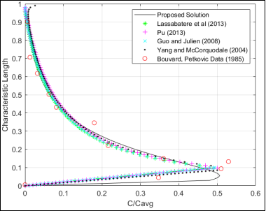
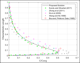
Figure 2. Proposed Sediment Concentration Solution Simulation (1a).

From figure 2, the proposed sediment concentration solution upholds a respectable holistic representation of the type II profile. The accuracy of the proposed solution performance varies with the change of characteristic length. Highlighting the

0.4 \leq ξ_{n} \leq 1

region, the proposed formulation accurately illustrates the near surface region and curvature of the suspended sediment concentration profile in accordance with the measured data

[2]

. Within the

0.1 \leq ξ_{n} \leq 0.3

region, the proposed solution captures the maximum concentration with significant accuracy; however, the formulation fails to accurately capture the characteristic length at which the maximum concentration occurs.

Table 3. Simulation (1a): Concentration MAE Analysis.

Concentration Mean Absolute Error (%)
Proposed Solution	Pu et al (2013)	Lassabatere et al (2013)	Guo and Julien (2008)	Yang and McCorquodale (2004)
0.29437488	0.88602377	0.64465944	0.851384889	0.9033337

Download: Download full-size image

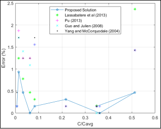
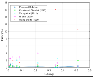
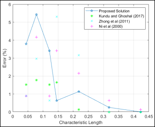
Figure 3. Simulation (1a): Concentration Error Analysis.

However, the proposed formulation can reflect the type II concentration profile under fully developed turbulent open channel flow conditions expressing an accuracy ranging from 46.15% to 99.63%. The proposed vertical velocity distribution (equation 37) provides the formularised concentration solution with reasonable correlation to the recorded data obtained from the literature

[2]

, confidently reflecting the maximum suspended sediment concentration region.

Download: Download full-size image

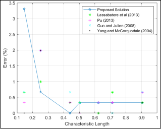
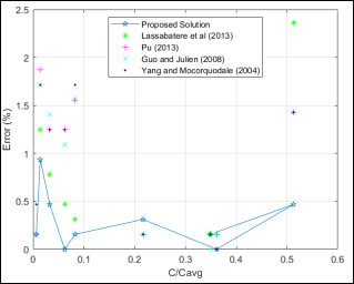
Figure 4. Simulation (1a): Characteristic Length Error Analysis.

Table 4. Simulation (1a): Characteristic Length MAE Analysis.

Characteristic Length Mean Absolute Error (%)
Proposed Solution	Pu et al (2013)	Lassabatere et al (2013)	Guo and Julien (2008)	Yang and McCorquodale (2004)
1.28773555	0.73908778	0.696181111	0.812665556	0.527393

From the characteristic length MAE analysis, the proposed solution holds accuracy within the near surface region and holds reasonable accuracy holistically. The proposed formulation showcased the highest characteristic length MAE, partially a consequence of the instability of the ‘

\ln (\frac{d_{z} - d_{z 0}}{k_{s}})

’ term found in equation (37)

[16]

To assess the capabilities of the proposed concentration solution to simulation conditions, validations against the established models are conducted

[10, 18, 24]

. Figures 5, 8, 11, and 14 are simulated from the data set provided in table 3. The proposed analytical quasi linear kinetic theory two-phase solid-liquid concentration profile solution is solved numerically using the 4^th order Runge-Kutta method. The laws of vertical distribution for dilute particles concentration are analysed from the angle of microscopic descriptions of mechanism based on kinetic theory of two-phase flow. The concentration profile evaluated is referred to as type II, where the sediment concentration increases initially with characteristic height, and achieves a maximum concentration at a distance from the bed; however, at the critical characteristic length the sediment concentration begins to decrease. From the analysis conducted it is essential to note that the particle-particle interactions, drift diffusion, time averaged mass and lift force are influential factors in presenting a type II concentration profile. Additionally, the lag velocity (

u_{l}^{+}

) and kinematic viscosity (

v_{fk}

) directly influence the curvature of the sediment suspension solution. In this analytical research the turbulence intensity of a particle is considered a function of flow depth rather than a constant. The proposed model reflects that the type II profile is achieved when the lift coefficient is increased, and a low Bulk Stokes Number is kept constant

[10]

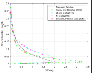
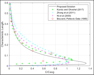
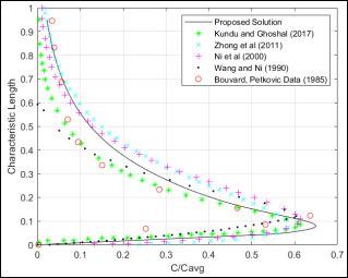
From figure 5, the proposed sediment concentration solution presented a strong correlation with the Bouvard and Petkovic (1985) data, depicting the near surface region and concentration curvature. As the characteristic length increases, the accuracy of the proposed solution also increases; this is due to the vertical velocity distribution formulations (equation 37) whereas when the vertical distance approaches zero the ‘

\ln (\frac{d_{z} - d_{z 0}}{k_{s}})

’ term becomes unstable, distorting the solution accuracy

[16]

. Evidently, this distortion has contributed to the proposed concentration solution’s inaccuracy in depicting the maximum concentration. It should be noted the Bouvard and Petkovic (1985) data displays anomalies (0.1808, 0.347682) and (0.5299, 0.135762) (simulation conditions and measured data is identical to that of figure 2).

Download: Download full-size image

Figure 5. Proposed Sediment Concentration Solution Simulation 1 (b).

Download: Download full-size image

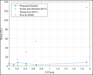
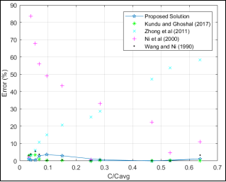
Figure 6. Simulation (1b): Concentration Error Analysis.

Table 5. Simulation (1b): Concentration MAE Analysis.

Concentration Mean Absolute Error (%)
Proposed Solution	Kundu and Ghoshal (2017)	Zhong et al (2011)	Ni et al (2000)	Wang and Ni (1990)
0.29437488	0.52021	1.1226074	1.9819214	3.9630457

With respect to the Bouvard and Petkovic (1985) data, the proposed solution accuracy ranges from 46.15% to 99.63%. The proposed hydrodynamic solution depicts the concentration with the lowest MAE results showcasing the proposed formulations’ capability in capturing the fluid-sediment behaviour against other established concentration solutions.

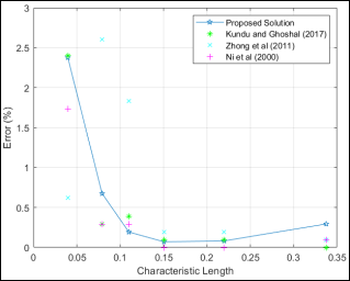
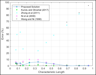
Table 6. Simulation (1b): Characteristic Length MAE Analysis.

Characteristic Length Absolute Error (%)
Proposed Solution	Kundu and Ghoshal (2017)	Zhong et al (2011)	Ni et al (2000)	Wang and Ni (1990)
1.287736	1.99577	2.81027	3.696314	12.42389

Download: Download full-size image

Figure 7. Simulation (1b): Characteristic Length Error Analysis.

From table 6, the proposed solution expressing the least characteristic length MAE depicting the type II concentration profile under fully developed turbulent open channel flow conditions. The characteristic length inaccuracy present is attributed to the sensitivity of the ‘

\ln (\frac{d_{z} - d_{z 0}}{k_{s}})

’ term incorporated into equation (37).

In this simulation, the conditions express an increase in sediment diameter while the settling velocity and shear velocity have decreased in respect to simulation (1). Importantly, the fluid shear velocity has decreased by more than half that expressed under simulation (1) conditions. From figure 8, the proposed sediment concentration solution presented strong correlation with the measured data set, depicting the near surface region and concentration curvature with reasonable accuracy. However, the proposed hydrodynamic solution is outperformed by the existing solution

[14, 24]

with regards to accurately depicting the maximum concentration and the characteristic length at which the maximum is achieved.

Download: Download full-size image

Figure 8. Proposed Sediment Concentration Solution Simulation (2).

Download: Download full-size image

Figure 9. Simulation (2): Concentration MAE Analysis Simulation.

The proposed concentration solution showcases an MAE less than that of Kundu and Ghoshal (2017), expressing an accuracy ranging from 40.47% to 99.63%. The overestimation of the sediment concentration expressed by the proposed solution is attributed to the assumption that the covariance of the fluid fluctuation velocities and the covariance of turbulence intensities being equal (

\overset{̅}{v_{f}^{'} v_{s}^{'}} = \overset{̅}{v_{f}^{' 2}}

)

[8, 10]

Table 7. Simulation (2): Concentration MAE Analysis.

Concentration Mean Absolute Error (%)
Proposed Solution	Kundu and Ghoshal (2017)	Zhong et al (2011)	Ni et al (2000)
5.3627133	23.14291667	5.203616167	18.263405

Table 8. Simulation (2): Characteristic Length MAE Analysis.

Characteristic Length Mean Absolute Error (%)
Proposed Solution	Kundu and Ghoshal (2017)	Zhong et al (2011)	Ni et al (2000)
0.615343	0.545165	0.923075	0.40101

Download: Download full-size image

Figure 10. Simulation (2): Characteristic Length Error Analysis.

With respect to simulation (1), the proposed concentration solution presented less inaccuracy in simulation (2). This is expressed along the profile curvature and within the near surface region attributed slight increase in sediment diameter. However, with respect to simulation (1), the maximum concentration depiction has decreased, reflecting a comprehensive limitation of the proposed solution and plausibility a consequence of the decreased shear velocity. From equation (37) due to the instability of the ‘

\ln (\frac{d_{z} - d_{z 0}}{k_{s}})

’ term the results of simulation (2) showcase an increase in inaccuracy as the characteristic length decreases. This behaviour is reflected under different simulation conditions highlighting the dimensionally comprehensive limitation of the proposed hydrodynamic formulation.

Download: Download full-size image

Figure 11. Proposed Sediment Concentration Solution Simulation (3).

Here, the simulation conditions express a relatively small increase in sediment diameter while the settling velocity and the shear velocity remain the same as that of simulation (2). When comparing simulation results from figures 5 and 11, the results indicate that under relatively low shear velocities, the proposed solution is not suited for relatively small sediment diameters. The near surface region and concentration curvature are depicted with reasonable accuracy, reflected by figure 11 illustrating the proposed sediment concentration solution capability. The maximum concentration has been overestimated, attributed to the assumption that the covariance of the fluid fluctuation velocities and the covariance of turbulence intensities being equal (

\overset{̅}{v_{f}^{'} v_{s}^{'}} = \overset{̅}{v_{f}^{' 2}}

)

[8, 10]

Table 9. Simulation (3): Concentration MAE Analysis.

Concentration Mean Absolute Error (%)
Proposed Solution	Kundu and Ghoshal (2017)	Zhong et al (2011)	Ni et al (2000)
31.67001129	7.82717	10.17003347	16.01748177

Download: Download full-size image

Figure 12. Simulation (3): Concentration Error Analysis.

It should be noted that the proposed concentration MAE has been significantly influenced by the maximum concentration results. In this simulation, against the remaining Bouvard and Petkovic data, the proposed solution performed reasonably well, achieving an accuracy of up to 99.82%. Similarly, to simulations (1) and (2), the maximum concentration depiction has decreased, again reflecting the instability within the proposed formulations to be attributed to the consequence of relatively low shear velocity conditions.

Download: Download full-size image

Figure 13. Simulation (3): Characteristic Length Error Analysis.

Table 10. Simulation (3): Characteristic Length MAE Analysis.

Characteristic Length Mean Absolute Error (%)
Proposed Solution	Kundu and Ghoshal (2017)	Zhong et al (2011)	Ni et al (2000)
2.093223	0.938344	1.848213	1.750376

From the MAE analysis, towards the bed the proposed solution presents greater inaccuracies with respect to the existing solutions

[10, 14, 24]

. However, as the characteristic length increases the error results decrease, expressed by the depiction of the concentration curvature and near surface region with reasonable accuracy, affirming the influence of the ‘

\ln (\frac{d_{z} - d_{z 0}}{k_{s}})

’ term.

Download: Download full-size image

Figure 14. Proposed Sediment Concentration Solution Simulation (4).

Here the simulation conditions express an increase in both the sediment diameter and shear velocity with respect to the preceding simulation conditions from table 3. From figure 14, the proposed sediment concentration solution with reasonable accuracy depicts the near surface region and the maximum concentration; however, within the

0.2 \leq ξ_{n} \leq 0.6

region, the proposed solution struggles to precisely capture the concentration curvature.

Download: Download full-size image

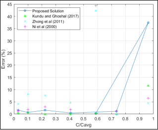
Figure 15. Simulation (4): Concentration Error Analysis.

Table 11. Simulation (4): Concentration MAE Analysis.

Concentration Mean Absolute Error (%)
Proposed Solution	Kundu and Ghoshal (2017)	Zhong et al (2011)	Ni et al (2000)	Wang and Ni (1990)
1.2585872	1.111213273	21.30247273	33.95057	0.802228182

Evidently, increasing the shear velocity and sediment diameter allows the solution to depict the maximum concentration more accurately. However, an overestimation of concentration is still exhibited, attributed to the assumption of (

\overset{̅}{v_{f}^{'} v_{s}^{'}} = \overset{̅}{v_{f}^{' 2}}

)

[7, 10]

Table 12. Simulation (4): Characteristic Length MAE Analysis.

Characteristic Length Mean Absolute Error (%)
Proposed Solution	Kundu and Ghoshal (2017)	Zhong et al (2011)	Ni et al (2000)	Wang and Ni (1990)
2.48825	0.64111	35.19331	3.694153	23.909736

Download: Download full-size image

Figure 16. Simulation (4): Characteristic Length Error Analysis.

Here the proposed solution can predict the type II concentration profile with accuracy up to 99.77%. Evidently, under relatively high shear velocities, the proposed solution expresses respectable characteristic length accuracy. Evidently, increasing the sediment diameter and shear velocity presents a decrease in the accuracy of the profile curvature.

5. Discussion

Evidently, with respect to the measured data, under relatively low shear velocity, increasing the sediment diameter allows for a clearer depiction of the near surface region and profile curvature. On the other hand, the proposed solution can accurately depict the near surface region, curvature of concentration, and maximum concentration under relatively large shear velocity data, with great accuracy as reflected from simulations (1) and (4). Importantly, under conditions where both the shear velocity and sediment diameter are relatively large, the maximum concentration is captured with greater accuracy, relative to that of the established solutions

[10, 24]

. solutions. However, under such conditions the holistic accuracy of the concentration profile (with respect to the profile curvature and near surface region) decreases, when compared to the results of simulations (2) and (3).

It is to be noted that as the characteristic length increases, the accuracy of the proposed solution also increases. This is due to the instability of the ‘

\ln (\frac{d_{z} - d_{z 0}}{k_{s}})

’ term as the vertical distance decreases to zero

[16]

. Additionally, the overestimation of the proposed concentration is attributed to the assumption that the covariance of the fluid fluctuating velocities and the covariance of turbulence intensities being equal (

\overset{̅}{v_{f}^{'} v_{s}^{'}} = \overset{̅}{v_{f}^{' 2}}

)

[5, 7, 10]

The Bouvard and Petkovic (1985) measured data is sparse, especially within the near wall region (i.e., figure 2). Experimental error is plausible as the measurements do not hold a quasi-linear form. From this, it should be acknowledged towards the bed, the definition of the maximum concentrations recorded from table 3 is not consistent enough to accurately conclude the proposed solution’s predictive ability. However, similar to other established solutions, under favourable simulation conditions (relatively high shear velocity) the proposed solution presents relative accuracy and can be used to provide insight to the near surface, curvature, and maximum concentrations under turbulent open channel flow conditions.

6. Conclusions

To contribute to the research field analytically through vertical velocity components, a novel formulation of the lift force is introduced by incorporating the bed roughness impact alongside the impact of secondary current induced vortices within the vertical velocity distribution (equation 37). The proposed 2D methodology is presented following the momentum equilibrium of group particle motion under uniform channel slope conditions. Implying that the sediment particles and the body of water are two separate sets of mass points with two different densities under laws of conservation of mass and momentum. From this both fluid and sediment particle inertia terms are eliminated, and the sediment concentration is reflected only from the vertical direction. The collision stresses are eliminated in this research under the assumption that particle-particle interactions are temporary and infrequent

[10, 24]

From this research, the lag velocity (u_l⁺) and kinematic viscosity (

v_{fk}

) contribute significantly to the quasi-linear curvature of the concentration profile. This research presented an alternative lift force solution, by incorporating the bed roughness height coefficient (

k_{s}

) within the lift force velocity distribution formulation (equation 37). Under favourable conditions, the proposed sediment concentration solution can reflect the maximum suspended sediment concentration, concentration curvature and concentrations within the near surface region with accuracy against the measured data setfrom table 3.

Abbreviations

B_r	Logarithmic Integration Constant
$c$	Dimensionless Celerity of a Small Disturbance
$C_{m}$	Maximum Volumetric Concentration in Particle Packing
$C_{D}$	Coefficient of Drag
$C_{L}$	Coefficient of Lift
d	Sediment Diameter
$D_{f}$	Damping of Fluid Turbulence due to Presences of Sediment
$D_{H}$	Hydraulic Diameter
$D_{s}$	Damping of Sediment Turbulence Relative to the Fluid
$d_{z}$	Dimensionless Flow Depth
e	Restitution Coefficient of Particle Collision
$f$	Flow Resistance
$f_{D}$	Darcy Weisbach Friction Factor
$F_{D}$	Drag Force
$F_{DL}$	Laminar Drag Force
$F_{DT}$	Turbulent Drag Force
$F_{L}$	Lift Force
$F_{sz}$	Particle Forces
$g_{0}$	Radial Distribution Function
$g_{z}$	Gravitational Acceleration Component in Respect to ‘z’
h	Incremental Interval Relative to the Flow Depth
$κ$	Clear Water von Karman Coefficient
$κ_{m}$	Sediment-Water Von Karman Coefficient
$k_{p}$	Turbulent Kinetic Energy of Sediments
$k_{s}$	Dimensionless Bed Roughness Height
$L_{y}$	Proposed Lift Force Per Unit Mass
MAE	Mean Average Error
$M_{sz}$	Proposed Modified Time Averaged Force
NBR	Near Bed Region
p	Water Pressure
$ρ_{s}$	Density of Sediment Phase
$ρ_{f}$	Density of Fluid Phase
$R$	Reynolds Number
${Re}_{d}$	Flow Reynolds Number
${Re}_{p}$	Particle Reynolds Number
$R_{s}$	Reynolds Shear Stress Generated due to Sediment Velocity Fluctuations
$S t_{b}$	Stokes Bulk Number
$t$	Dimensionless Time
$U_{c}$	Flow Celerity
$u_{c}$	Dimensionless Flow Celerity
$u_{d}$	Drift Velocity
$u_{f}$	Mean Velocity of Fluid Along the Streamwise Direction
$u_{l}$	Lag Velocity
$u_{n}$	Proposed Resolved Flow Celerity
$u_{r}$	Relative Velocity
$u_{s}$	Instantaneous Particle Velocity Components in Respect to ‘x’
$u_{*}$	Shear Velocity
$v_{f}$	Vertical Velocity of the Fluid Phase
$v_{fk}$	Kinematic Viscosity
$v_{n}$	Proposed Resolved Flow Velocity
$v_{r}^{2}$	Relative Velocity of a Sediment to the Fluid
$v_{s}$	Instantaneous Particle Velocity Components in Respect to ‘z’
x	Streamwise Dimension
$x_{h}$	Hydraulic Jump Height Location
$x_{s}$	Wave Front Tip Location
z	Vertical Dimension
$ε_{f}$	Fluid Eddy Viscosity
$ε_{n}$	Proposed Resolved Shockwave Velocity
$ε_{s}$	Sediment Diffusivity Coefficient
$ε_{w}$	Shockwave Velocity
$ξ_{n}$	Characteristic Length Function
$σ_{s}$	Particle Stress
$ξ_{t}$	Proposed Bed Roughness Height incorporated Characteristic Length Function
µ	Dynamic Viscosity
$τ_{p}$	Ratio of the Relative Particle Velocity to a Particle Timescale
$τ_{t}$	Net Drag Force Due to Turbulent Motion
$\overset{̅}{v_{f}^{' 2}}$	Turbulence Intensity of the Fluid Phase
$\overset{̅}{v_{s}^{' 2}}$	Turbulence Intensity of the Solid Phase
$ω_{0}$	Sediment Settling Velocity
$γ$	Proportionality Constant based on the Inverse of the Turbulent Schmidt Number
Π	Coles Wake Parameter
$σ_{s}$	Particle Stress
$Φ$	Function of Vertical Distance
$θ_{p}$	Proposed Resolve Angle
θ	Bed slope Angle
$φ$	Polygama Function defines the (n+1)^th Derivative of a Logarithm
$Ψ (ξ_{t, n})$	Proposed Characteristic Length Function

Author Contributions

Tarek Taha is the sole author. The author read and approved the final manuscript.

Data Availability Statement

The data supporting the outcome of this research work has been reported in this manuscript.

Conflicts of Interest

The author declares no conflicts of interest.

References

[1]	Auton T. R., (1987). “The lift force on a spherical body in a rotational flow”. Journal of Fluid Mechanics, 183: 199-218. https://doi.org/10.1017/S002211208700260X
[2]	Bouvard M, Petkovic S, (1985). Vertical dispersion of spherical, heavy particles in turbulent open channel flow.” Journal of Hydraulic Research, 23(1): 5-20. https://doi.org/10.1080/00221688509499373
[3]	Celik I, and Gel A, (2002). “A new approach in modeling phase distribution in fully developed bubble pipe flow”. Flow Turbulence and Combustion, 68: 289-311. https://doi.org/10.1023/A:1021765605698
[4]	Chen X, Li Y, Zhang Z, (2018). “Effective Nikuradse Roughness on the Mobile Plan Bed”. China Ocean Engineering, 32: 730-736. https://doi.org/10.1007/s13344-018-0074-1
[5]	Greimann BP, Holly FM, (2001). “Two-phase analysis of concentration profiles”. Journal of Hydraulic Engineering, 127(9): 753-762. https://doi.org/10.1061/(ASCE)0733-9429(2001)127:9(753)
[6]	Guo J, Julien, Y. P., (2008). “Application of the Modified Log Wake Law in Open Channels”. Journal of Applied Fluid Mechanics, 1(2): 17-23. https://doi.org/10.36884/JAFM.1.02.11844
[7]	Jha K, Bombardelli F. A., (2010). “Toward two-phase flow modeling of nondilute sediment transport in open channels”. Journal of Geophysical Reserch, 115: 1-27. https://doi.org/10.1029/2009JF001347
[8]	Jiang JS, Law A. W. K., Cheng N. S., (2004). “Two-phase modeling of suspended sediment distribution in open channel flows”. Journal of Hydraulic Research 42(3): 273-281. https://doi.org/10.1080/00221686.2004.9728392
[9]	Kundu S, Ghoshal K (2014). “Effects of secondary current and stratification on suspension concentration in an open channel flow”. Journal of Environmental Fluid Mechanics, 14(6): 1357-1380. https://doi.org/10.1007/s10652-014-9341-8
[10]	Kundu S, Ghoshal K, (2017). “A mathematical model for type II concentration distribution in turbulent flows”. Journal of Environmental Fluid Mechanics, 17: 449-472. https://doi.org/10.1007/s10652-016-9498-4
[11]	Lassabatere L, Pu J. H., Bonakdari H, Joannis C, Larrarte F, (2013). “Velocity Distribution In Open Channel Flows: Analytical Approach for the Outer Region”. American Society of Civil Engneers, Volume 139(1): 37-43. https://doi.org/10.1061/(ASCE)HY.1943-7900.0000609
[12]	Liu Q. Q., Shu A. P., Singh V. P., (2007). “Analysis of the Vertical Profile of Concentration in Sediment-Laden Flows”. Journal of Engineering Mechanics, 133(6): 601-607. https://doi.org/10.1061/(ASCE)0733-9399(2007)133:6(601)
[13]	Mustaffa N, Ahmad N. A., Razi M. A., (2016). “Variations of Roughness Coefficients with Flow Depth of Grassed Swale.” Langkawi, Malaysia, Soft Soil Engineering International Conference, 1-7. https://doi.org/10.1088/1757-899X/136/1/012082
[14]	Ni J. R., Wang G. Q., Borthwick A. G. L., (2000). “Kinetic theory for particles in dilute and dense solid-liquid flows.” Journal of Hydraulic Engineering, 126(12): 893-903. https://doi.org/10.1061/(ASCE)0733-9429(2000)126:12(89)
[15]	Nikuradse J, (1993). “Laws of Flow in Rough Pipes”. National Advisory Committee for Aeronautics Report No. 1292, Springer-VDI Verlag, Vol. 361.
[16]	Pu J. H., (2013). “Universal Velocity Distribution for Smooth and Rough Open Channel Flows.” Journal of Applied Fluid Mechanics, 6(3): 413-423. https://doi.org/10.36884/jafm.6.03.21301
[17]	Toorman A, (2008). “Vertical mixing in the fully developed turbulent layer of sediment-laden open-channel flow.” Journal of Hydraulic, Engineering, 134(9), 1225-1235. https://doi.org/10.1061/(ASCE)0733-9429(2008)134:9(122)
[18]	Wang G. Q., Ni J. R., (1990). “Kinetic theory for particle concentration distribution in two-phase flows.” Journal of Engineering Mechanics, 116(12): 2738-2748. https://doi.org/10.1061/(ASCE)0733-9399(1990)116:12(2738)
[19]	Yang S. Q., McCorquodale J. A., (2014). “Determination of Boundary Shear Stress and Reynolds Shear Stress in Smooth Rectangular Channel Flows.” Journal of Hydraulic Engineering, 130(5): 458-462. https://doi.org/10.1061/(ASCE)0733-9429(2004)130:5(458)
[20]	Yang S. Q., Tan S. K., Lim S. Y., (2004). “Velocity distribution and dip-phenomenon in smooth uniform open channel flows.” Journal of Hydraulic Engeernig, 130(12): 1179-1186. https://doi.org/10.1061/(ASCE)0733-9429(2004)130:12(1179)
[21]	Yang S. G., (2007). “Turbulent transfer mechanism in sediment-laden flow.” Journal of Geophysical Research, 112: 10051-14. https://doi.org/10.1029/2005JF000452
[22]	Young J, and Leeming A, (1997). “A theory of particle deposition in turbulent pipe flow.” Journal of Fluid Mechanics., 340: 129-159. https://doi.org/10.1017/S0022112097005284
[23]	Zhang L. W. H., (2015). “Numerical simulation of dam-break flows using a TVD finite-volume method with wet-dry fronts capturing.” Journal of Hydrodynamics, 27(5): https://doi.org/10.1002/hyp.6242
[24]	Zhong D, Wang G, Sun Q, (2011). “Transport equation for suspended sediment based on two-fluid model of solid/liquid two-phase flows.” Journal of Hydraulic Research, 137(5): 530-542. https://doi.org/10.1061/(ASCE)HY.1943-7900.0000331

Cite This Article

Plain Text BibTeX RIS

APA Style

Taha, T. (2024). Bed Roughness Incorporated Lift Force Formulation for Sediment Concentration Solutions. American Journal of Water Science and Engineering, 10(1), 8-26. https://doi.org/10.11648/j.ajwse.20241001.12

Copy | Download

ACS Style

Taha, T. Bed Roughness Incorporated Lift Force Formulation for Sediment Concentration Solutions. Am. J. Water Sci. Eng. 2024, 10(1), 8-26. doi: 10.11648/j.ajwse.20241001.12

Copy | Download

AMA Style

Taha T. Bed Roughness Incorporated Lift Force Formulation for Sediment Concentration Solutions. Am J Water Sci Eng. 2024;10(1):8-26. doi: 10.11648/j.ajwse.20241001.12

Copy | Download

@article{10.11648/j.ajwse.20241001.12,
  author = {Tarek Taha},
  title = {Bed Roughness Incorporated Lift Force Formulation for Sediment Concentration Solutions
},
  journal = {American Journal of Water Science and Engineering},
  volume = {10},
  number = {1},
  pages = {8-26},
  doi = {10.11648/j.ajwse.20241001.12},
  url = {https://doi.org/10.11648/j.ajwse.20241001.12},
  eprint = {https://article.sciencepublishinggroup.com/pdf/10.11648.j.ajwse.20241001.12},
  abstract = {Within the field of sediment transport dynamics, there is an emphasis on the need for providing and improving simplified analytical solutions from which the findings can be extended upon. Typically, solutions have been developed from the understanding and incorporation of vertical velocity components/distribution; however, there remains opportunity for analytical enhancement. Under uniform open channel dilute sediment laden flow conditions, the type II concentration profile reflects the maximum concentration at a distance from the bed. To analytically depict the type II profile, it is essential to describe the vertical velocity components acting within the flow hydrodynamics. Yet, the impact of bed roughness on the vertical velocity distribution influencing a sediment particle has not been articulated. Hence, in this research, the impact of bed roughness is incorporated into the vertical velocity distribution to formulate the lift force acting upon a particle, to provide a sediment concentration solution. The proposed analytical vertical velocity distribution solution is validated against existing formulations, followed by the proposed sediment concentration being validated against existing solutions. Here, the results indicate that analytically incorporating the bed roughness alongside the secondary current induced vortices provides a lift force solution that can depict the type II concentration profile. Under relatively low shear velocity, increasing the sediment diameter allows for a clearer depiction of the near surface region and profile curvature. Furthermore, the proposed sediment concentration solution can accurately depict the near surface region, curvature of concentration, and maximum concentration under relatively large shear velocity data. Importantly, under conditions where both the shear velocity and sediment diameter are relatively large, the maximum concentration is captured with greater accuracy; however, the curvature of the profile and the near surface region accuracy are hindered. It is to be noted, that due to the formulation of the proposed velocity distribution the accuracy of the solution towards the bed decreases due to instability caused as the characteristic depth decreases to zero.
},
 year = {2024}
}

Copy | Download

TY  - JOUR
T1  - Bed Roughness Incorporated Lift Force Formulation for Sediment Concentration Solutions

AU  - Tarek Taha
Y1  - 2024/08/06
PY  - 2024
N1  - https://doi.org/10.11648/j.ajwse.20241001.12
DO  - 10.11648/j.ajwse.20241001.12
T2  - American Journal of Water Science and Engineering
JF  - American Journal of Water Science and Engineering
JO  - American Journal of Water Science and Engineering
SP  - 8
EP  - 26
PB  - Science Publishing Group
SN  - 2575-1875
UR  - https://doi.org/10.11648/j.ajwse.20241001.12
AB  - Within the field of sediment transport dynamics, there is an emphasis on the need for providing and improving simplified analytical solutions from which the findings can be extended upon. Typically, solutions have been developed from the understanding and incorporation of vertical velocity components/distribution; however, there remains opportunity for analytical enhancement. Under uniform open channel dilute sediment laden flow conditions, the type II concentration profile reflects the maximum concentration at a distance from the bed. To analytically depict the type II profile, it is essential to describe the vertical velocity components acting within the flow hydrodynamics. Yet, the impact of bed roughness on the vertical velocity distribution influencing a sediment particle has not been articulated. Hence, in this research, the impact of bed roughness is incorporated into the vertical velocity distribution to formulate the lift force acting upon a particle, to provide a sediment concentration solution. The proposed analytical vertical velocity distribution solution is validated against existing formulations, followed by the proposed sediment concentration being validated against existing solutions. Here, the results indicate that analytically incorporating the bed roughness alongside the secondary current induced vortices provides a lift force solution that can depict the type II concentration profile. Under relatively low shear velocity, increasing the sediment diameter allows for a clearer depiction of the near surface region and profile curvature. Furthermore, the proposed sediment concentration solution can accurately depict the near surface region, curvature of concentration, and maximum concentration under relatively large shear velocity data. Importantly, under conditions where both the shear velocity and sediment diameter are relatively large, the maximum concentration is captured with greater accuracy; however, the curvature of the profile and the near surface region accuracy are hindered. It is to be noted, that due to the formulation of the proposed velocity distribution the accuracy of the solution towards the bed decreases due to instability caused as the characteristic depth decreases to zero.

VL  - 10
IS  - 1
ER  -

Copy | Download

Author Information

Tarek Taha

Civil Engineering, Leeds College of Building University Centre, Leeds, United Kingdom

Biography: Tarek Taha is a fluid dynamics and open channel researcher and a lecturer at Leeds College of Building University Centre. Contributed to the Journal of Environmental Fluid Mechanics, Academics World 2019 International Conference and Fluid Mechanics Research International Journal.

Research Fields: Fluid mechanics, open channel, dilute flow, dam break flow, vertical velocity components, sediment concentration, quantitative 3D turbulent structure evaluation, hydrodynamics.

Contact Email

http://orcid.org/0009-0007-9214-4333

Download PDF

Plain Text BibTeX RIS

APA Style

Taha, T. (2024). Bed Roughness Incorporated Lift Force Formulation for Sediment Concentration Solutions. American Journal of Water Science and Engineering, 10(1), 8-26. https://doi.org/10.11648/j.ajwse.20241001.12

Copy | Download

ACS Style

Taha, T. Bed Roughness Incorporated Lift Force Formulation for Sediment Concentration Solutions. Am. J. Water Sci. Eng. 2024, 10(1), 8-26. doi: 10.11648/j.ajwse.20241001.12

Copy | Download

AMA Style

Taha T. Bed Roughness Incorporated Lift Force Formulation for Sediment Concentration Solutions. Am J Water Sci Eng. 2024;10(1):8-26. doi: 10.11648/j.ajwse.20241001.12

Copy | Download

@article{10.11648/j.ajwse.20241001.12,
  author = {Tarek Taha},
  title = {Bed Roughness Incorporated Lift Force Formulation for Sediment Concentration Solutions
},
  journal = {American Journal of Water Science and Engineering},
  volume = {10},
  number = {1},
  pages = {8-26},
  doi = {10.11648/j.ajwse.20241001.12},
  url = {https://doi.org/10.11648/j.ajwse.20241001.12},
  eprint = {https://article.sciencepublishinggroup.com/pdf/10.11648.j.ajwse.20241001.12},
  abstract = {Within the field of sediment transport dynamics, there is an emphasis on the need for providing and improving simplified analytical solutions from which the findings can be extended upon. Typically, solutions have been developed from the understanding and incorporation of vertical velocity components/distribution; however, there remains opportunity for analytical enhancement. Under uniform open channel dilute sediment laden flow conditions, the type II concentration profile reflects the maximum concentration at a distance from the bed. To analytically depict the type II profile, it is essential to describe the vertical velocity components acting within the flow hydrodynamics. Yet, the impact of bed roughness on the vertical velocity distribution influencing a sediment particle has not been articulated. Hence, in this research, the impact of bed roughness is incorporated into the vertical velocity distribution to formulate the lift force acting upon a particle, to provide a sediment concentration solution. The proposed analytical vertical velocity distribution solution is validated against existing formulations, followed by the proposed sediment concentration being validated against existing solutions. Here, the results indicate that analytically incorporating the bed roughness alongside the secondary current induced vortices provides a lift force solution that can depict the type II concentration profile. Under relatively low shear velocity, increasing the sediment diameter allows for a clearer depiction of the near surface region and profile curvature. Furthermore, the proposed sediment concentration solution can accurately depict the near surface region, curvature of concentration, and maximum concentration under relatively large shear velocity data. Importantly, under conditions where both the shear velocity and sediment diameter are relatively large, the maximum concentration is captured with greater accuracy; however, the curvature of the profile and the near surface region accuracy are hindered. It is to be noted, that due to the formulation of the proposed velocity distribution the accuracy of the solution towards the bed decreases due to instability caused as the characteristic depth decreases to zero.
},
 year = {2024}
}

Copy | Download

TY  - JOUR
T1  - Bed Roughness Incorporated Lift Force Formulation for Sediment Concentration Solutions

AU  - Tarek Taha
Y1  - 2024/08/06
PY  - 2024
N1  - https://doi.org/10.11648/j.ajwse.20241001.12
DO  - 10.11648/j.ajwse.20241001.12
T2  - American Journal of Water Science and Engineering
JF  - American Journal of Water Science and Engineering
JO  - American Journal of Water Science and Engineering
SP  - 8
EP  - 26
PB  - Science Publishing Group
SN  - 2575-1875
UR  - https://doi.org/10.11648/j.ajwse.20241001.12
AB  - Within the field of sediment transport dynamics, there is an emphasis on the need for providing and improving simplified analytical solutions from which the findings can be extended upon. Typically, solutions have been developed from the understanding and incorporation of vertical velocity components/distribution; however, there remains opportunity for analytical enhancement. Under uniform open channel dilute sediment laden flow conditions, the type II concentration profile reflects the maximum concentration at a distance from the bed. To analytically depict the type II profile, it is essential to describe the vertical velocity components acting within the flow hydrodynamics. Yet, the impact of bed roughness on the vertical velocity distribution influencing a sediment particle has not been articulated. Hence, in this research, the impact of bed roughness is incorporated into the vertical velocity distribution to formulate the lift force acting upon a particle, to provide a sediment concentration solution. The proposed analytical vertical velocity distribution solution is validated against existing formulations, followed by the proposed sediment concentration being validated against existing solutions. Here, the results indicate that analytically incorporating the bed roughness alongside the secondary current induced vortices provides a lift force solution that can depict the type II concentration profile. Under relatively low shear velocity, increasing the sediment diameter allows for a clearer depiction of the near surface region and profile curvature. Furthermore, the proposed sediment concentration solution can accurately depict the near surface region, curvature of concentration, and maximum concentration under relatively large shear velocity data. Importantly, under conditions where both the shear velocity and sediment diameter are relatively large, the maximum concentration is captured with greater accuracy; however, the curvature of the profile and the near surface region accuracy are hindered. It is to be noted, that due to the formulation of the proposed velocity distribution the accuracy of the solution towards the bed decreases due to instability caused as the characteristic depth decreases to zero.

VL  - 10
IS  - 1
ER  -

Copy | Download