Accuracy Assessment of Dimensionality Reduction Techniques in Novel Approach of Precise Noise Levels Prediction and Mapping

Peter Ekow Baffoe; Yao Yevenyo Ziggah

doi:doi:10.11648/j.ajnna.20241001.12

Research Article |

| Peer-Reviewed

Accuracy Assessment of Dimensionality Reduction Techniques in Novel Approach of Precise Noise Levels Prediction and Mapping

Peter Ekow Baffoe^*

, Yao Yevenyo Ziggah

Published in American Journal of Neural Networks and Applications (Volume 10, Issue 1)

Received: 11 April 2024 Accepted: 6 May 2024 Published: 24 May 2024

Views: Downloads:

Download PDF

Share This Article

Twitter
Linked In
Facebook

Abstract

The increasing effects of noise pollution have necessitated the prediction of noise levels. In this regard, it has become very prudent to find models which are practically applicable and have the capability to predict noise levels with accuracy. In this project, two dimensionality reduction techniques namely the Principal Component Analysis (PCA) and Partial Least Squares (PLS) were used in truncating the dimensions of observed noise levels data collected in the Tarkwa Mining Community (TMC) for which the data with reduced dimensions served as input data for a Back Propagation Neural Network noise prediction model. The accuracies of the techniques were determined using statistical indicators. The Partial Least Squares technique had a better accuracy with RMSE of 1.135 when hybridized with the Back Propagation Neural Network. The performance of the Principal Component Analysis was also with RMSE of 1.373 and that of the observed noise data produced an RMSE of 1.433. Graphical representations also showed the precision of individual predicted noise levels compared to the observed noise levels. The importance of the techniques used in predicting noise levels cannot be overemphasized based on the results obtained.

Published in	American Journal of Neural Networks and Applications (Volume 10, Issue 1)
DOI	10.11648/j.ajnna.20241001.12
Page(s)	15-26
Creative Commons	This is an Open Access article, distributed under the terms of the Creative Commons Attribution 4.0 International License (http://creativecommons.org/licenses/by/4.0/), which permits unrestricted use, distribution and reproduction in any medium or format, provided the original work is properly cited.
Copyright	Copyright © The Author(s), 2024. Published by Science Publishing Group

Keywords

Noise Level Prediction, Noise Mapping, Dimensionality Reduction Techniques, Back Propagation Neural Network

1. Introduction

Humans are prone to all kinds of hazards. Noise comes as no exception to the number of hazards the human race face. In fact, man has lived with noise from time immemorial. Noise is an unwanted sound judged to be unpleasant, loud or disruptive to hearing. Noise evolves from various sources, some of which can be completely controlled and others, which are created from sudden happenings of natural phenomena become daunting a task to curtail. Taking into consideration the intense noise that comes with volcanic eruption, thunderstorms and other phenomena of its ilk.

Noise is also generated by the engine and exhaust systems of vehicles by aerodynamic systems and by interaction between the vehicle and its supporting systems

[15]

. From all the aforementioned sources, it is evident that noise generation and its effects are inevitable and their complete eradication from the social environment is fairly impossible in this present time. Sound perception by humans is in the range of 20 Hz to 20 kHz but the ear is far more sensitive to sound in the ranges of 1 kHz and 4 kHz

[14]

, above which is detrimental to hearing.

Noise has been considered to be only an accident product of human undertakings, but just a few years back, authorities decided to catalogue and deal with this canker. Noise pollution is currently more dominant in the mining communities at an alarming rate. This is due to a number of factors, some of which include infrastructural development, social development and high influx of people from different cultural backgrounds, with implication of increased generation of noise

[3]

An array of literature suggests and confirm that noise pollution does not only cause hearing impairment, also psychological disorders, interference with speech, sleep disorders, damaged brain and an effect on job performance as about 30 million people are exposed to high sound levels on their jobs in the United States

[6]

. It is worthy to note that commercial areas experience the highest noise levels, industrial areas follow, then residential areas fall lowest at the pecking order as reported by

[5]

. The Tarkwa Mining community shares these characteristics especially in its commercial areas where mining activities, movement of vehicles and trade between inhabitants breed unpleasant sound. From noise produced during the excavation of overburden, loading and dumping and transport, to sound from vehicle horns and loud music played on and along streets, accompanied with the cacophony of noise created by traders when undertaking their business ventures, noise pollution continuous to emanate intensely in the mining communities.

The United States Environmental Protection Agency suggests that noise above 80 decibels are detrimental to the human health, of which children are susceptible to noise above 60 decibels

[7]

. Also, the average noise levels in mine sites fall between 90 dBA and 150 dBA on mining floors based on preliminary analyses reported by

[4]

. This gives evidence of the high noise levels produced in the Tarkwa Mining Community.

With all the stated causes and effects, it is of much essence for noise levels to be predicted not only to find remedies to control the menace of noise pollution in the environment but also to aid in the urban planning and development. Albeit many studies been done with regards to the use of modern techniques such as Neural Networks in predicting noise levels

[8-11]

it can be stated that prediction of noise levels using dimensionality reduction techniques

[1, 2, 12]

, such as Principal Component Analysis (PCA) and Partial Least Squares (PLS) in conjunction with the Back Propagation Neural Network (BPNN) in precise prediction of traffic noise levels have not been explored and their capabilities have not been duly ascertained in this regard. Hence there is the need for the use of these modern techniques in predicting noise levels. Therefore, in this particular study future noise pollution levels were predicted using the Principal Component Analysis and the Partial Least Squares in conjunction with the Back Propagation Neural Network.

2. Materials and Methods Used

2.1. Study Area

Tarkwa is the capital of the Tarkwa-Nsuaem Municipal area, a Municipality in the Western Region southwest of South Ghana. The area has an average height of about 70 meters and known to be undulating. The peak of the elevation ranges from 150 and 300 meters above sea level

[2]

. The town is noted as a center of Gold and manganese mining. The number of mining companies cluster between the villages of Aboso and Tamso

[16]

. The Tarkwa Mine has the distinction of being one of the largest gold mines in the world. Approximately 24 tonnes of Gold is produced annually and 100 million tons of earth is moved to achieve this production rate

[13]

Download: Download full-size image

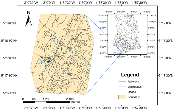
Figure 1. Tarkwa Mining Area.

Due to the number of mining activities in the area, a number of people who are not indigenes have come to reside in the town for a number of purposes some of which include employment, businesses and trade. This has increased the number of transport systems in the area since there is the need for movement from place to place. Cars being the main means of transportation for the inhabitants. The area has an average climate condition of 25 degrees Celsius. Over the past few years, the Tarkwa community has experienced tremendous infrastructural developments including road constructions, building of health posts, education, industries, banking, hospitality services and private business

[3]

. Figure 1 shows the study area as inserted in the map of Ghana.

2.2. Field Data Collection

The geo-spatial locations of the purpose-designed monitoring stations (PMS) in the TMC were surveyed using Garmin GPS 60CSx handheld Global Positioning System (GPS) of 2 m accuracy. A calibrated Larson Davis’s SoundTrack LxT Sound Level Meter was used to measure the noise levels in the study area. The measurements of the PMS were taken at street level and were also determined with the aid of the city digital map. To avoid noise reflections, the noise-level meter was set on a tripod at about 1.5 m above the ground level and separated from the noise sources by at least 1.5 m. This decision was made in connection with what has been reported and accepted in the literature. For example, in

[16]

used 1.5 m above ground level and 1.22-1.52 m from the source of the noise. The tolerance of the calibrated Larson Davis’s Sound Track LxT trademark device is ±0.6 dBA. A-weighted instantaneous sound pressure levels were recorded three times daily at the selected positions in the study area. The total number of the points used for the modelling was 50.

2.3. Methods Used

2.3.1. Partial Least Squares

The Partial Least Squares is a method that has been applied in many fields of science. It also takes up the name projection to latent structure due to its functionality. In the method, latent factors are determined based on the dependent and independent variables. The term latent explains the fact that though the factors are hidden, they explain much of an information about a particular subject or technically, a variable. Basically, it tries to determine the best components which can explain much information in both the dependent and independent variables.

The scores for the data ‘t_a’ and ‘u_a’ in the X and Y space respectively were computed using the equations expressed in Equations (1) and (2):

t_{a} = X_{a} v_{a}

(1)

u_{a} = Y_{a} f_{a}

(2)

The scores extracted needed to fulfill the three objectives as explained with the maximum covariance between them. The proceeding mathematical expression was used in computing the covariance as in Equation (3):

cov (t_{a}, u_{a}) = \frac{\sum \{(ta - {\overset{̅}{t}}_{a}) (u_{a} - {\overset{̅}{u}}_{a})\}}{n - 1}

(3)

The scores were found subject to the constraint that the loadings when summed up would result in giving a unit length. In making analysis and interpreting scores, though there are two sets of scores which are computed, the t-scores are used due to the fact that they are easily interpretable and readily available. The reason behind neglecting the u-scores during interpretation and analysis is based on the foundation that the u-scores are only available when the dependent variable is known.

2.3.2. Principal Component Analysis

The Principal Component Analysis is a technique used in finding patterns in data. Once the patterns of the data are determined, the data can be compressed i.e. the dimension(s) of the data can be reduced without losing much information

[12]

The eigen values were determined employing the algebraic expression stated in Equation (4):

|A - λI| = 0

(4)

The covariance between the independent variables were determined as represented by ‘A’ above, after which the identity matrix was constructed. The determinant was then computed to obtain the eigen values. The corresponding eigen vectors were obtained using the formula expressed in Equation (5):

(A - λI) X = 0

(5)

The determination of the eigen values and vectors allowed for the most important components to be chosen. The Non-Iterative Partial Least Square algorithm (NIPALS) which is a cross validation technique assists in giving the number of components which explain much of the variance in the data but the components to be chosen is based on the discretion of the analyst.

The values which constitute the Eigen vectors when summed gave a unit length which is a constraint that needs to be satisfied. The eigen vectors which also takes the name loadings were used in transforming the data to obtain the scores. The scores are the projection of the data onto the principal components. Each principal component consists of the scores and the eigen vector. The transformed data is computed using the equation expressed in Equation (6):

Z=X*U(6)

Where, X is a matrix of the original data, U being the eigen vectors or principal components chosen and Z the scores or a transformation matrix in a lower n-dimensional space.

2.3.3. Back Propagation Neural Network

The Back Propagation Neural Network was used as a predictive model for the exercise. The model is a well-known algorithm in the deep learning environment and it serves the purpose of training feedforward neural networks for supervised learning. The model needed a number of ingredients in order to generate the results required. To achieve this, the data obtained from PCA, PLS and the whole scaled data were segregated into parts where the majority of it about 70% was used as the training data and the 30% of the data was used to validate and test the model. The model requires an input data for which forms the basis for prediction and target data which would be the yardstick for which the outputs determined would be compared. Five (5) input neurons, 10 neurons in the hidden layer and an output neuron characterized the model for prediction. The Levenberg Marquardt algorithm was used for the training and the LEARNGDM was the gradient descent used as the adaption learning function in MATLAB. The performance function used was the mean square error (MSE) with the transfer function being the TANSIG chosen based on its ability to solve nonlinear problems. The mean square error was computed for each technique and also for the dimensionally unreduced data to enable the determination of their performance.

2.3.4. Model Accuracy Assessment

To ascertain the accuracies of the models, the statistical indicators listed below were adopted based on the equations depicted from Equation 7 to Equation 8. The equations are indicators helping to make fair evaluation of the models and they include Root Mean Square (RMSE), R² which is coefficient of determination, Data Scaling, R is correlation coefficient, mean and Standard Deviation.

zXi=(Xi-

\overset{̅}{x}

)/Std(X)(7)

zYi=(Yi-

\overset{̅}{x}

)/Std(Y)(8)

Equation (9) was used in scaling the predictor variables, to ensure a zero mean and a unit standard deviation. The scaled data augmented the computation of the correlation coefficient, R.

R_x,y=

Σ

[zXi*zYi]/n-1(9)

Where n is the number of observations, Oi and Pi being observed and predicted data respectively with the difference providing the errors. The Root Mean Square was computed using Equation (10).

RMSE=

\sqrt{\frac{\sum_{i = 1}^{n} {(O_{i} - P_{i})}^{2}}{n}}

(10)

The dependent variable, the observed noise levels, were centered using Equation (11).

y_{i} = Y_{i} - \overset{̅}{y}

(11)

3. Results and Discussion

3.1. Results Obtained After Prediction

Table 1 displays the errors obtained using both hybridized models on the primary data. It also displays predicted noise levels for both models.

Table 1. Predicted Noise Levels with Associated Errors.

Observed	Observed (Centred)	Predicted (PCA)	Error (PCA)	Predicted (PLS)	Error (PLS)
65	-20.2245	-17.2029	-3.0216	-20.2245	0.0000
78	-7.2245	-6.7765	-0.448	-7.2241	-0.0004
84	-1.2245	-0.6589	-0.5656	-0.2013	-1.0232
84	-1.2245	0.1041	-1.3286	-1.2249	0.0004
75	-10.2245	-10.141	-0.0835	-10.2246	0.0001
86	0.7755	2.1905	-1.415	0.7754	0.0001
79	-6.2245	-6.7765	0.552	-7.2241	0.9996
88	2.7755	2.7992	-0.0237	2.7758	-0.0003
85	-0.2245	0.0805	-0.305	0.2759	-0.5004
86	0.7755	0.0805	0.695	0.2759	0.4996
89	3.7755	4.6571	-0.8816	1.5378	2.2377
90	4.7755	4.6571	0.1184	1.5378	3.2377
91	5.7755	5.8973	-0.1218	5.7508	0.0247
98	12.7755	12.2568	0.5187	12.6617	0.1138
96	10.7755	8.2406	2.5349	12.7685	-1.9930
94	8.7755	10.7517	-1.9762	8.5991	0.1764
83	-2.2245	-1.6951	-0.5294	-1.2266	-0.9979
81	-4.2245	-2.449	-1.7755	-4.2289	0.0044
84	-1.2245	-1.6951	0.4706	-1.2266	0.0021
85	-0.2245	-0.0421	-0.1824	-0.2238	-0.0007
75	-10.2245	-10.2298	0.0053	-10.2239	-0.0006
76	-9.2245	-10.2298	1.0053	-10.2239	0.9994
74	-11.2245	-10.2298	-0.9947	-10.2239	-1.0006
77	-8.2245	-6.8932	-1.3313	-7.2241	-1.0004
79	-6.2245	-6.8932	0.6687	-7.2241	0.9996
74	-11.2245	-12.8798	1.6553	-11.7244	0.4999
73	-12.2245	-12.8798	0.6553	-11.7244	-0.5001
86	0.7755	0.7813	-0.0058	0.7772	-0.0017
88	2.7755	4.3186	-1.5431	2.7765	-0.0010
84	-1.2245	-3.1993	1.9748	-1.226	0.0015
89	3.7755	5.5993	-1.8238	6.2817	-2.5062
87	1.7755	2.0958	-0.3203	1.8026	-0.0271
89	3.7755	5.1805	-1.405	4.7766	-1.0011
90	4.7755	5.1805	-0.405	4.7766	-0.0011
95	9.7755	11.0214	-1.2459	11.6161	-1.8406
98	12.7755	10.1008	2.6747	10.8753	1.9002
97	11.7755	11.0214	0.7541	11.6161	0.1594
87	1.7755	0.8545	0.921	1.7757	-0.0002
86	0.7755	0.8545	-0.079	1.7757	-1.0002
89	3.7755	6.6165	-2.841	3.7719	0.0036
93	7.7755	7.9642	-0.1887	8.7675	-0.9920
95	9.7755	7.9642	1.8113	8.7675	1.0080
94	8.7755	5.5993	3.1762	6.2817	2.4938
96	10.7755	10.1008	0.6747	10.8753	-0.0998
92	6.7755	5.1805	1.595	4.7766	1.9989
88	2.7755	1.8495	0.926	2.7764	-0.0009
80	-5.2245	-6.8932	1.6687	-7.2241	1.9996
76	-9.2245	-6.8932	-2.3313	-7.2241	-2.0004
68	-17.2245	-17.211	-0.0135	-17.2224	-0.0021

Table 2. Accuracy Assessment of Models using Statistical Indicators.

Model	Standard Deviation	Mean	RMSE	R²
PCA-BPNN	1.386138	-0.04348	1.135	0.984
PLS-BPNN	1.144861	0.058541	1.373	0.987

RMSE = Root Mean Square Error, R² = Coefficient of Correlation

Table 3. Summary of Principal Component Analysis.

Components	R²X	R²X (Cumul.)	Eigenvals.	Q²	Limit	Q² (Cumul.)
1	0.45837	0.45837	2.29184	0.2201	0.21667	0.2201
2	0.26572	0.72409	1.32859	0.20066	0.26596	0.3766

Table 4. Principal Component with their Corresponding Eigenvalues and Variance.

Component	Eigenvalue	Percentage of Variance (%)	Cumulative Variance (%)
1	2.29194	45.84	45.84
2	1.32852	26.57	72.41
3	0.69895	13.98	86.39
4	0.58166	11.63	98.02
5	0.09893	1.98	100.00

Table 5. Coefficients of Principal Components.

Predictors	Coefficients of PC1	Coefficients of PC2
POP	-0.45426	0.35983
Traffic	0.51782	0.26625
Road net.	-0.0031	0.74152
Land use	0.4031	0.43554
Dist.	0.60251	-0.24511

Table 6. Loadings of Predictors on Principal Components.

Predictors	PC1	PC2
POP	0.693273	0.404026
Traffic	-0.779713	0.309337
Road net.	0.015944	0.859016
Land use	-0.603578	0.505647
Dist.	-0.915805	-0.275817

Download: Download full-size image

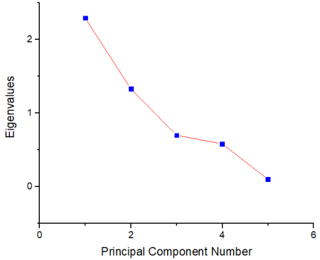
Figure 2. Scree Plot Displaying PCs and Eigenvalues.

Download: Download full-size image

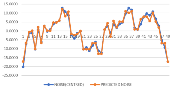
Figure 3. A Graph of Predicted and Observed Noise Levels using PCA.

Download: Download full-size image

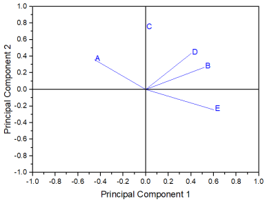
Figure 4. Loadings in PCA.

Table 7. Summary of Partial Least Squares.

Number of Factors	Variance Explained for X Effects (%)	Cumulative x variance (%)	Variance Explained for Y Responses (%)	Cumulative y variance (%)
1	42.8286	42.8286	56.39184	56.39184
2	27.67881	70.50741	9.98528	66.37712
3	5.19388	75.7013	26.75447	93.13159
4	11.49075	87.19205	2.89362	96.02521
5	12.80795	100	0.02797	96.05318

Table 8. Partial Least Squares Loadings.

Predictors	Factor 1	Factor 2
POP	-5.43909	0.51595
Traffic	4.35257	3.1581
Road net.	-2.33731	5.24753
Land use	2.40894	5.27832
Dist.	6.55699	0.89002

Download: Download full-size image

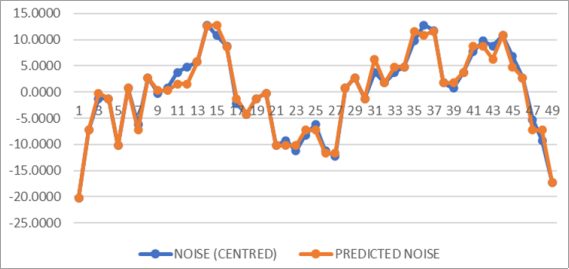
Figure 5. A Graph of Predicted and Observed Noise Levels Using PLS.

Download: Download full-size image

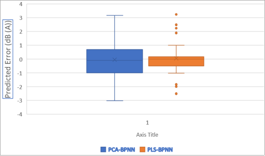
Figure 6. Box and Whisker Plots of Model Errors.

Download: Download full-size image

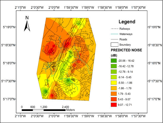
Figure 7. Noise Map of the Study Area After Prediction.

3.2. Discussion

Dimensionality reduction on the observed data using the Principal Component Analysis provided a number of Principal Components for which the first two sets of scores served as input for the Back Propagation Neural Network. The two components were selected based on the notion that the first and second components contributed 46% and 27% to the total variance. A cumulative of about 73%. The scree plot in Figure 2 shows a sharp bend after the third component and it is not entirely out of place to add the third component but from the table, the third component contributes very little to the variance and that justifies why it was not selected. A moderately concrete justification could also be stated to support the argument of selecting two components. This is with respect to the Eigenvalues obtained for both components. An inference from Table 4 gives the eigenvalues 2.29 and 1.32 for the first and second components and the rest less than 1.

One might think that the reason for ignoring the other three components was as a result of the absence of their importance but that would not be a right justification for that attempt. In totality, all the components contributed to the makeup of the total variance but the whole concept is to reduce the dimensions of the data such that the components which carry much variance are selected to explain the data and thus to provide ease of analyses and visualization.

The coefficients obtained in Table 5 showed how each of the five predictors or independent variables contributed to the Principal Components. Basically, the coefficients express the influence of each predictor on the Principal Components. In PC1, distribution, traffic and land use show positive correlation between them and from Table 6, the predictor variable (population) loads strongly on PC1. It was realized that a negative correlation existed between population and road network in PC1. Rightly so, an increase in distribution in a given area reduces the population in the area and an increase in land use decreases road network and vice versa.

In PC2, population, traffic, road network and land use have a positive correlation with one another where road network contribute strongly as compared to land use whose influence is fairly strong and slightly above the other predictor variables. Road network in PC2, loaded strongly when compared to the other predictor variables.

In the Partial Least Squares, two factors were used with a cumulative of 66% in the dependent variable and 71% in the independent variables. As explained earlier, the Partial Least Squares finds the factor(s) which explain much of the variance in both the outcome variable (y) and the predictor variables (x). In Table 8, the predictor variables, distribution and traffic load heavily on factor 1 whilst road network and land use load heavily on factor 2.

Figure 6 displays the box and whisker plots for the error distribution after prediction. The upper and lower whiskers depict maximum and minimum errors for both methods respectively. The outliers as seen predominantly above and below the whiskers of the PLS-BPNN were determined using the 1.5 IQR rule. It is realized that the PLS-BPNN had a narrow interquartile range, proving less variability in the PLS-BPNN compared to the PCA-BPNN.

Root Mean Square Error computed for the Principal Component Analysis, Partial Least Squares and the unreduced data were 1.373, 1.135 and 1.433 respectively. The PLS-BPNN produced a better RMSE chiefly due to its ability to incorporate the dependent variable in determining the factors. The data showing the predicted values, errors, the computed Root Mean Square Errors for all the methods among other results are displayed in the appendix.

Figure 7 displays the map of the study area using the predicted noise levels from the PLS-BPNN. The map shows areas experiencing very high noise levels and it could be inferred that these areas are the mining areas where their activities breed such noise. The results proved that these areas experienced over 65 dba of noise levels which is above the Environmental Protection Agency standards, and as such poses health risk to inhabitants. The areas which experience such low noise levels is as a result of the less dense demographics and low trade activities in the area.

4. Conclusion

Every data can be displayed in its inherent dimensions based on its characteristic variables and any method which becomes effective in eliminating redundant dimensions to ensure easy visualization and processing should be utilized. The Principal Component Analysis and Partial Least Squares were used in truncating the dimensions of the noise data and the resultant data served as inputs into a Back Propagation Neural Network. The accuracies of these methods based on their performance using the observed noise levels dataset were assessed after the process. The PCA determined components which explained much information (variance) in the data by providing associated eigenvalues whilst the Partial Least Squares provided factors which explained much information in the dataset using both the dependent and independent variables.

The observed noise level data used as input for the Back Propagation Neural Network provided the least accuracy, with RMSE of 1.433 as compared to when both the Principal Component Analysis, 1.373 and the Partial Least Squares 1.135 when used on the Neural Network independently. The methods used in truncating the dimensions of the data allowed for easy training, testing and validation together with reducing learning time and improved the accuracy of the Artificial Neural Network. This can be assessed in the regression models obtained for each method.

For better data analysis and visualization, it is very essential that methods which provide optimum results are used in reducing the dimensions of the data. This does not only eliminate redundant information from the data, it also helps simplifies the analysis to be done.

Abbreviations

PCA	Principal Component Analysis
PLS	Partial Least Square
BPNN	Back Propagation Neural Network
TMC	Tarkwa Mining Community

Author Contributions

Peter Ekow Baffoe: Conceptualization, Data curation, Investigation, Methodology, Project administration, Supervision, Validation, Writing – original draft, Writing – review & editing

Yao Yevenyo Ziggah: Data curation, Investigation, Methodology, Project administration, Supervision, Validation, Visualization, Writing – original draft, Writing – review & editing

Conflicts of Interest

The authors declare no conflicts of interest.

References

[1]	Ali, I., Wasif, K. and Bavomi, H. (2024), “Dimensionality Reduction for Images loT using Machine Learning”, Earth Environment and Planetary Sciences, Vol. 40, pp. 47-61.
[2]	Anowar, F., Samira, S., and Selim, B. (2023), “Conceptual and Empirical Comparison of Dimensionality Reduction Algorithm’.
[3]	Baffoe, P. E., and Duker, A. A. (2019), “Evaluation of Two Noise Level Prediction Models: Multiple Linear Regression and a Hybrid Approach”, American Journal of Mathematical and Computer Modelling. Vol. 4, No. 3, pp. 91-99.
[4]	Bauer, E. R., Kohler, J. L. (2000), “Cross sectional Survey of Noise Exposure in the Mining Industry”, National Institute for Occupational Safety and Health Office of Mine Safety and Health Research, Publication No. 76, pp. 2-15.
[5]	Braj, B., and Jain, V. K. (1995), “A Comparative Study of Noise Levels in Some Residential, Industrial and Commercial Areas of Delhi”, Environmental Monitoring and Assessment, Vol. 35, pp. 1-11.
[6]	Chepesiuk, R. (2005), “Decibel Hell: The Effects of Living in a Noisy World”, Environmental Health Perspectives, Vol. 113, No. 1, pp. 35 - 37.
[7]	Elezaj, R., (2019), “Noise Pollution Effects: What Do You Think It Does to Humans?”, Health Europa, 7^th Ed., Grosag Publication, Vancouver, 2pp.
[8]	Genaro N., Torija A., Ramos-Ridao A., Requena, I., Ruiz D. P., and Zamorano M. (2010), “A Neural Network-Based Model for Urban Noise Prediction”, The Journal of the Acoustical Society of America, Vol. 128, pp. 1738-1746.
[9]	Hamad, K., Khalilb, M., and Shanableha, A. (2017), “Modeling Roadway Traffic Noise in A Hot Climate Using Artificial Neural Networks” Transportation Research Part D: Transport and Environment, Vol. 53, pp. 161-177.
[10]	Kumar, K., Parida, M., and Katiyar, V. K. (2012), “Artificial Neural Network Modeling for Road Traffic Noise Prediction”, Third International Conference on Computing, Communication and Networking Technologies, pp. 3-5.
[11]	Nedic, V., Despotovic, B., and Cvetanovic S. (2014), “Comparison of Classical Statistical Methods and Artificial Neural Network in Traffic Noise Prediction”, Environmental Impact Assessment Review, Vol. 49, pp. 24-30.
[12]	Rafieian, B., Hermosilla, P. and Vazquez, P. P. (2023), “Improving Dimensionality Reduction Projections for Data Visualization”, Appl. Sci., Vol. 13 (17), 9967: https://doi.org/10.3390/app13179967
[13]	Shillington, K (2012). “History of Africa”, London: Palgrave Macmillan. pp. 93–94.
[14]	Smith, A. (2003), “Effects of Noise, Job Characteristics and Stress on Mental Health and Accidents, Injuries and Cognitive Failures at Work”, International Commission on Biological Effects of Noise, pp. 1-6.
[15]	Sukeerth G., Munilakshmi N. and Anilkumarreddy C. (2017), “Mathematical Modeling for the Prediction of Road Traffic Noise Levels in Tirupati Town”, International Journal of Engineering Development and Research, Vol. 5, pp. 2091-2097.
[16]	Wright, J. B., Hastings, D. A., Jones, W. B., Williams, H. R. (1985). “Geology and Mineral Resources of West Africa”, London: George Allen & UNWIN, pp. 45–47.

Cite This Article

Plain Text BibTeX RIS

APA Style

Baffoe, P. E., Ziggah, Y. Y. (2024). Accuracy Assessment of Dimensionality Reduction Techniques in Novel Approach of Precise Noise Levels Prediction and Mapping. American Journal of Neural Networks and Applications, 10(1), 15-26. https://doi.org/10.11648/j.ajnna.20241001.12

Copy | Download

ACS Style

Baffoe, P. E.; Ziggah, Y. Y. Accuracy Assessment of Dimensionality Reduction Techniques in Novel Approach of Precise Noise Levels Prediction and Mapping. Am. J. Neural Netw. Appl. 2024, 10(1), 15-26. doi: 10.11648/j.ajnna.20241001.12

Copy | Download

AMA Style

Baffoe PE, Ziggah YY. Accuracy Assessment of Dimensionality Reduction Techniques in Novel Approach of Precise Noise Levels Prediction and Mapping. Am J Neural Netw Appl. 2024;10(1):15-26. doi: 10.11648/j.ajnna.20241001.12

Copy | Download

@article{10.11648/j.ajnna.20241001.12,
  author = {Peter Ekow Baffoe and Yao Yevenyo Ziggah},
  title = {Accuracy Assessment of Dimensionality Reduction Techniques in Novel Approach of Precise Noise Levels Prediction and Mapping
},
  journal = {American Journal of Neural Networks and Applications},
  volume = {10},
  number = {1},
  pages = {15-26},
  doi = {10.11648/j.ajnna.20241001.12},
  url = {https://doi.org/10.11648/j.ajnna.20241001.12},
  eprint = {https://article.sciencepublishinggroup.com/pdf/10.11648.j.ajnna.20241001.12},
  abstract = {The increasing effects of noise pollution have necessitated the prediction of noise levels. In this regard, it has become very prudent to find models which are practically applicable and have the capability to predict noise levels with accuracy. In this project, two dimensionality reduction techniques namely the Principal Component Analysis (PCA) and Partial Least Squares (PLS) were used in truncating the dimensions of observed noise levels data collected in the Tarkwa Mining Community (TMC) for which the data with reduced dimensions served as input data for a Back Propagation Neural Network noise prediction model. The accuracies of the techniques were determined using statistical indicators. The Partial Least Squares technique had a better accuracy with RMSE of 1.135 when hybridized with the Back Propagation Neural Network. The performance of the Principal Component Analysis was also with RMSE of 1.373 and that of the observed noise data produced an RMSE of 1.433. Graphical representations also showed the precision of individual predicted noise levels compared to the observed noise levels. The importance of the techniques used in predicting noise levels cannot be overemphasized based on the results obtained.
},
 year = {2024}
}

Copy | Download

TY  - JOUR
T1  - Accuracy Assessment of Dimensionality Reduction Techniques in Novel Approach of Precise Noise Levels Prediction and Mapping

AU  - Peter Ekow Baffoe
AU  - Yao Yevenyo Ziggah
Y1  - 2024/05/24
PY  - 2024
N1  - https://doi.org/10.11648/j.ajnna.20241001.12
DO  - 10.11648/j.ajnna.20241001.12
T2  - American Journal of Neural Networks and Applications
JF  - American Journal of Neural Networks and Applications
JO  - American Journal of Neural Networks and Applications
SP  - 15
EP  - 26
PB  - Science Publishing Group
SN  - 2469-7419
UR  - https://doi.org/10.11648/j.ajnna.20241001.12
AB  - The increasing effects of noise pollution have necessitated the prediction of noise levels. In this regard, it has become very prudent to find models which are practically applicable and have the capability to predict noise levels with accuracy. In this project, two dimensionality reduction techniques namely the Principal Component Analysis (PCA) and Partial Least Squares (PLS) were used in truncating the dimensions of observed noise levels data collected in the Tarkwa Mining Community (TMC) for which the data with reduced dimensions served as input data for a Back Propagation Neural Network noise prediction model. The accuracies of the techniques were determined using statistical indicators. The Partial Least Squares technique had a better accuracy with RMSE of 1.135 when hybridized with the Back Propagation Neural Network. The performance of the Principal Component Analysis was also with RMSE of 1.373 and that of the observed noise data produced an RMSE of 1.433. Graphical representations also showed the precision of individual predicted noise levels compared to the observed noise levels. The importance of the techniques used in predicting noise levels cannot be overemphasized based on the results obtained.

VL  - 10
IS  - 1
ER  -

Copy | Download

Author Information

Peter Ekow Baffoe

Geomatic Engineering Department, University of Mines and Technology, Tarkwa, Ghana

Contact Email

http://orcid.org/0000-0002-2659-034X
Yao Yevenyo Ziggah

Geomatic Engineering Department, University of Mines and Technology, Tarkwa, Ghana

Contact Email

http://orcid.org/0000-0002-9940-1845

Download PDF

Plain Text BibTeX RIS

APA Style

Baffoe, P. E., Ziggah, Y. Y. (2024). Accuracy Assessment of Dimensionality Reduction Techniques in Novel Approach of Precise Noise Levels Prediction and Mapping. American Journal of Neural Networks and Applications, 10(1), 15-26. https://doi.org/10.11648/j.ajnna.20241001.12

Copy | Download

ACS Style

Baffoe, P. E.; Ziggah, Y. Y. Accuracy Assessment of Dimensionality Reduction Techniques in Novel Approach of Precise Noise Levels Prediction and Mapping. Am. J. Neural Netw. Appl. 2024, 10(1), 15-26. doi: 10.11648/j.ajnna.20241001.12

Copy | Download

AMA Style

Baffoe PE, Ziggah YY. Accuracy Assessment of Dimensionality Reduction Techniques in Novel Approach of Precise Noise Levels Prediction and Mapping. Am J Neural Netw Appl. 2024;10(1):15-26. doi: 10.11648/j.ajnna.20241001.12

Copy | Download

@article{10.11648/j.ajnna.20241001.12,
  author = {Peter Ekow Baffoe and Yao Yevenyo Ziggah},
  title = {Accuracy Assessment of Dimensionality Reduction Techniques in Novel Approach of Precise Noise Levels Prediction and Mapping
},
  journal = {American Journal of Neural Networks and Applications},
  volume = {10},
  number = {1},
  pages = {15-26},
  doi = {10.11648/j.ajnna.20241001.12},
  url = {https://doi.org/10.11648/j.ajnna.20241001.12},
  eprint = {https://article.sciencepublishinggroup.com/pdf/10.11648.j.ajnna.20241001.12},
  abstract = {The increasing effects of noise pollution have necessitated the prediction of noise levels. In this regard, it has become very prudent to find models which are practically applicable and have the capability to predict noise levels with accuracy. In this project, two dimensionality reduction techniques namely the Principal Component Analysis (PCA) and Partial Least Squares (PLS) were used in truncating the dimensions of observed noise levels data collected in the Tarkwa Mining Community (TMC) for which the data with reduced dimensions served as input data for a Back Propagation Neural Network noise prediction model. The accuracies of the techniques were determined using statistical indicators. The Partial Least Squares technique had a better accuracy with RMSE of 1.135 when hybridized with the Back Propagation Neural Network. The performance of the Principal Component Analysis was also with RMSE of 1.373 and that of the observed noise data produced an RMSE of 1.433. Graphical representations also showed the precision of individual predicted noise levels compared to the observed noise levels. The importance of the techniques used in predicting noise levels cannot be overemphasized based on the results obtained.
},
 year = {2024}
}

Copy | Download

TY  - JOUR
T1  - Accuracy Assessment of Dimensionality Reduction Techniques in Novel Approach of Precise Noise Levels Prediction and Mapping

AU  - Peter Ekow Baffoe
AU  - Yao Yevenyo Ziggah
Y1  - 2024/05/24
PY  - 2024
N1  - https://doi.org/10.11648/j.ajnna.20241001.12
DO  - 10.11648/j.ajnna.20241001.12
T2  - American Journal of Neural Networks and Applications
JF  - American Journal of Neural Networks and Applications
JO  - American Journal of Neural Networks and Applications
SP  - 15
EP  - 26
PB  - Science Publishing Group
SN  - 2469-7419
UR  - https://doi.org/10.11648/j.ajnna.20241001.12
AB  - The increasing effects of noise pollution have necessitated the prediction of noise levels. In this regard, it has become very prudent to find models which are practically applicable and have the capability to predict noise levels with accuracy. In this project, two dimensionality reduction techniques namely the Principal Component Analysis (PCA) and Partial Least Squares (PLS) were used in truncating the dimensions of observed noise levels data collected in the Tarkwa Mining Community (TMC) for which the data with reduced dimensions served as input data for a Back Propagation Neural Network noise prediction model. The accuracies of the techniques were determined using statistical indicators. The Partial Least Squares technique had a better accuracy with RMSE of 1.135 when hybridized with the Back Propagation Neural Network. The performance of the Principal Component Analysis was also with RMSE of 1.373 and that of the observed noise data produced an RMSE of 1.433. Graphical representations also showed the precision of individual predicted noise levels compared to the observed noise levels. The importance of the techniques used in predicting noise levels cannot be overemphasized based on the results obtained.

VL  - 10
IS  - 1
ER  -

Copy | Download