Scaling Point-Based Habitat Observations of Anopheles stephensi Using XGBoost to Support Seek-and-Destroy Larval Source Management in Kisumu, Kenya

Odelia Asher; Rishil Shah; Aarya Satardekar; Anusha Parajuli; Namit Choudhari; James Jedrzejczyk; Joseph Mwangangi; Charles Mbogo; Benjamin Jacob

doi:doi:10.11648/j.aje.20261003.11

Research Article |

Scaling Point-Based Habitat Observations of Anopheles stephensi Using XGBoost to Support Seek-and-Destroy Larval Source Management in Kisumu, Kenya

Odelia Asher^*, Rishil Shah, Aarya Satardekar, Anusha Parajuli, Namit Choudhari, James Jedrzejczyk, Joseph Mwangangi, Charles Mbogo, Benjamin Jacob

Published in American Journal of Entomology (Volume 10, Issue 3)

Received: 17 June 2026 Accepted: 1 July 2026 Published: 6 August 2026

Views: Downloads:

Download PDF

Share This Article

Twitter
Linked In
Facebook

Abstract

The invasive malaria vector Anopheles stephensi poses an emerging challenge to malaria control in rapidly urbanizing regions of East Africa. This study evaluates the spatial distribution and potential spread of An. stephensi across Kisumu County by integrating field entomological observations with machine learning models applied to satellite-derived environmental data. The primary objective was to scale habitat signatures identified at confirmed georeferenced capture locations to the county level to support a targeted “Seek-and-Destroy” larval source management (S&D-LSM) strategy. Confirmed larval and adult capture points were used to extract environmental predictors from 10-m resolution visible and near-infrared (IR) bands derived from Sentinel-2 imagery. These spectral variables, along with derived indices representing vegetation structure, surface moisture, and urban disturbance, served as input features for predictive modeling. Three ensemble machine learning approaches—Random Forest, Gradient Boosting, and Extreme Gradient Boosting (XGBoost)—were implemented to model the relationship between environmental signatures and observed mosquito presence. Each model was trained using capture locations and background samples to classify potential breeding habitats across the landscape. Model performance was evaluated using cross-validation and standard classification metrics, and the resulting predictions were used to generate habitat suitability maps for the entirety of Kisumu County. Ensemble tree methods effectively captured nonlinear relationships between spectral features and mosquito habitat conditions, enabling the identification of spatial clusters of high-probability breeding environments. XGBoost achieved the highest predictive performance (AUC = 0.96), demonstrating superior ability to quantify complex nonlinear relationships and interactions among environmental and anthropogenic An. stephensi predictors. The eigen-autocorrelation statistics revealed a Moran’s Index of -0.159, a variance of 0.005, a z-score of 0.019 and a p-value of 0.04. Areas of elevated suitability were frequently associated with dense settlement patterns, infrastructure corridors, and locations with intermittent water storage or container habitats. The resulting risk surfaces enabled vector control teams to prioritize surveillance and intervention efforts. By spatially targeting activities toward high-probability sites, the program operationalized an S&D-LSM approach focused on rapid detection and elimination of breeding habitats. This study demonstrates that integrating remote sensing with ensemble machine learning provides a scalable framework for monitoring invasive malaria vectors and supporting targeted urban malaria control interventions.

Published in	American Journal of Entomology (Volume 10, Issue 3)
DOI	10.11648/j.aje.20261003.11
Page(s)	45-61
Creative Commons	This is an Open Access article, distributed under the terms of the Creative Commons Attribution 4.0 International License (http://creativecommons.org/licenses/by/4.0/), which permits unrestricted use, distribution and reproduction in any medium or format, provided the original work is properly cited.
Copyright	Copyright © The Author(s), 2026. Published by Science Publishing Group

Keywords

An. stephensi, Sentinel-2 Imagery, XGBoost, Eigen-autocorrelation Kisumu, Kenya

1. Introduction

Malaria is an infectious parasitic disease transmitted to humans through the bite of infected female Anopheles mosquitoes carrying Plasmodium parasites

[1]

. Malaria is endemic in the lake and coastal regions of Kenya, including Kisumu County, which is in western Kenya. The main vectors of malaria transmission that have been identified in western Kenya include Anopheles gambiae s.s, An. arabiensis, and An. funestus, s.l.

[2, 3]

. The An. stephensi mosquito is an emerging vector in Kenya that was first detected on the African continent in Djibouti in 2012

[4]

. Since then, it has been reported in different African countries such as Sudan and Ethiopia in 2016, Somalia in 2019, Nigeria in 2020, and Ghana, Kenya, and Eritrea in 2022

[4]

. Researchers suggest that An. stephensi may have found its way into Kenya through major highways that connect Kenya to Ethiopia and South Sudan

[5]

Three biological forms of An. stephensi have been described: type, intermediate, and mysorensis. Among these, the type form is primarily associated with urban environments and is considered the most efficient malaria vector, whereas the mysorensis form is predominantly found in rural settings and exhibits comparatively lower vector competence

[6]

Compared with native African malaria vectors, An. stephensi exhibits distinct ecological and behavioral characteristics, including both zoophilic and anthropophilic host preferences and a tendency to rest in animal shelters. Unlike native vectors that typically breed in clean natural water bodies in rural settings, An. stephensi can utilize both clean and polluted water in natural and artificial containers, particularly within urban environments

[7, 11]

In western Kenya, the urban and peri-urban landscapes of Kisumu County present a complex mosaic of built infrastructure, informal settlements, wetlands, and peri-agricultural land uses that can facilitate the proliferation of container-breeding mosquito species

[8]

. According to Yousefi, et al.

[9]

, larval habitats of An. stephensi in Iran are defined by temporary man-made habitats. Furthermore, access to water bodies, propitious temperatures ranging from 20C to 30C, and sunny unshaded areas had a positive correlation with the oviposition of An. stephensi mosquitoes

[8]

. These characteristics are geographically in place with Kisumu County, which is in the basin of the largest lake in Africa, Lake Victoria, and experiences a range of moderate temperatures

[10]

An. stephensi has also demonstrated a remarkable ability to colonize densely populated urban environments by exploiting artificial water containers, rooftop tanks, construction sites, and other anthropogenic habitats

[4, 11]

. Its establishment in countries across the region has raised significant concern among public health agencies due to its potential to sustain malaria transmission in urban settings that were previously considered relatively low risk

[4]

In 2023, the population at risk for malaria infections in Kenya was 55,339,002, with 1,060 reported deaths

[2]

. In response, various insecticides, which are used in indoor residual spraying (IRS) and selected long-lasting insecticidal nets (LLINs), have been used to control malaria vectors

[10]

. However, it has been reported that An. stephensi exhibits resistance to pyrethroids, organochlorines, carbamates, organophosphates, dichlorodiphenyltrichloroethane (DDT), and malathion, which are some of the insecticides used for mosquito control

[9, 10]

. With such outcomes, identifying larval habitats of An. stephensi might be much more effective in reducing the incidence and mortality rates of malaria

[9]

Conventional vector surveillance approaches rely heavily on field-based larval habitat inspections and localized entomological surveys

[8]

. While these methods provide high-quality observations, they are spatially limited and resource-intensive, making it difficult to scale surveillance and intervention strategies across entire administrative regions.

Advances in satellite remote sensing together with modern machine learning techniques have substantially improved our ability to characterize environmental conditions associated with mosquito breeding habitats. Satellite platforms such as Sentinel-2 offer high-frequency multispectral imagery at spatial resolutions capable of detecting environmental conditions associated with mosquito breeding habitats. When combined with field observations, these datasets can be used to characterize spectral and environmental signatures associated with known vector habitats. Machine learning algorithms are particularly well suited for modeling such relationships, as they can capture complex nonlinear interactions between environmental variables and species occurrence.

Ensemble tree-based approaches—including Random Forest, Gradient Boosting, and XGBoost—have demonstrated strong performance in ecological classification and habitat suitability modeling. These methods combine the predictions of several base estimators built with a given learning algorithm to improve generalizability and robustness over a single estimator. These algorithms can integrate large sets of spectral predictors and derived environmental indices while maintaining robustness to noise and variable interactions.

This study integrates field entomological observations with multispectral satellite data to model and scale habitat signatures of An. stephensi across Kisumu County. By training ensemble machine learning models on environmental features extracted from confirmed capture locations, we generated spatial predictions of potential larval habitats across the county. The resulting habitat suitability surfaces support an operational “Seek-and-Destroy” larval source management (S&D-LSM) framework that prioritizes high-probability breeding locations for targeted surveillance and intervention. Our assumption was that through this approach, we could demonstrate how remote sensing and machine learning can enhance vector surveillance capacity and support scalable control strategies for invasive malaria vectors in rapidly urbanizing environments.

The aims of this paper were to construct a Poisson count variable probability model, spectrally extrapolate varying An. stephensi habitat signatures from georeferenced capture points to the county level using geospatial and machine learning libraries, and employ a second-order eigen decomposition eigen-autocorrelation specification weights matrix to regressively forecast aggregation and non-aggregation oriented, i.e., hot and cold spot sites, in Kisumu, Kenya. The geospatial and machine learning libraries utilized included GeoPandas for spatial data processing, Rasterio for satellite imagery extraction, Scikit-learn for Random Forest, Gradient Boosting models, and XGBoost for large-scale spatial prediction of georeferenceable hot and cold spot stratified clusters.

2. Materials and Methods

Kisumu is the third-largest city in Kenya located in the Lake Victoria area in the former Nyanza Province. It is the second-largest city in the Lake Victoria Basin after Kampala. The city has a population of 438,588 according to the recent 2026 population estimates. The metro region, including Maseno and Ahero, had a population of 6,771 (Maseno) and 11,801 (Ahero) people respectively, totaling to a combined population of 457,160 people, according to the 2019 Kenya Population and Housing Census, which was conducted by the Kenya National Bureau of Statistics. Kisumu's elevation is 1,131 m (3,711 ft) and is about 320 km (200 mi) northwest of Nairobi, on the shores of Lake Victoria. It lies at the northeastern edge of the Winam Gulf, a long, shallow arm that protrudes from the main body of Lake Victoria

[9]

. Kisumu is 24 km (15 mi) south of the equator and has, due to its elevation, moderate temperatures. Kisumu features a tropical rainforest climate with no true dry season and significant rainfall year-round. January is the driest month, while the month of April receives the most rainfall. Kisumu has highly fertile land and variations in temperature and rainfall, with two rainy seasons per year across the region providing a suitable environment for a broad range of agricultural crops. The Kisumu region has approximately 1.6 million hectares of agricultural land. However, it is estimated that only 58 percent of the land is currently used. The majority of farming in the lake basin region is subsistence agriculture, leading to relatively low production volume

[9]

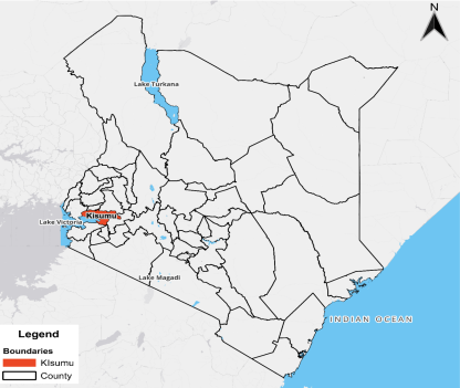
2.1. Study Site Map of Kisumu

Download: Download full-size image

Figure 1. Kisumu County.

2.2. Satellite Data

We created a LULC map of Kisumu using the 10-meter visible and near-IR (infrared) imagery. We first acquired cloud-free Level-2A surface reflectance data from the European Space Agency covering the Kisumu metropolitan region and surrounding agricultural landscape near Lake Victoria. The key 10-m bands—blue (B2), green (B3), red (B4), and near-infrared (IR) (B8)—are stacked and preprocessed with atmospheric correction, cloud masking, and clipping to the study boundary. (Table 1)

Table 1. Sentinel-2 with spectral bands at different spatial resolutions.

Band Number	Sentinel-2A		Sentinel-2B		Spatial resolution (m)
Band Number	Central wavelength (nm)	Bandwidth (nm)	Central wavelength (nm)	Bandwidth (nm)	Spatial resolution (m)
1	442.7	20	442.3	20	60
2	492.7	65	492.3	65	10
3	559.8	35	558.9	35	10
4	664.6	30	664.9	31	10
5	704.1	14	703.8	15	20
6	740.5	14	739.1	13	20
7	782.8	19	779.7	19	20
8	832.8	105	832.9	104	10
8a	864.7	21	864.0	21	20
9	945.1	19	943.2	20	60
10	1373.5	29	1376.9	29	60
11	1613.7	90	1610.4	94	20
12	2202.4	174	2185.7	184	20

Training samples representing urban surfaces (dense buildings and roads in central Kisumu), peri-urban transition zones with mixed housing and vegetation, and rural farmland dominated by cropland and smallholder fields were collected from high-resolution reference imagery using field entomological sampling data. A supervised classification algorithm (i.e., maximum likelihood) was applied to classify the stacked spectral bands and indices into the three land-cover categories. Accuracy assessment included remotely validating the predicted georeferenced capture points to evaluate the reliability of the map and post-processing (such as smoothing and removing isolated pixels). This rendered a final 10-m resolution land-use map distinguishing urban, peri-urban, and rural farmland zones. 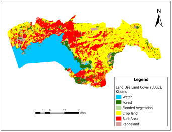We assumed these An. stephensi regression maps would enable implementing a S&D-LSM program. The LULC-classified map revealed the capture points and surface area (m²) of each site, including remote, sampled, georeferenced, stratified sentinel sites, as well as potential An. stephensi habitats (Figure 2).

Download: Download full-size image

Figure 2. LULC Map of Kisumu County.

2.3. Regression Model

Initially, a Poisson regression with statistical significance was calculated at a 95% confidence level in R. The Poisson process in our analysis was provided by the limit of a binomial distribution of the larval sampled An. stephensi habitat estimator determinants. Table 1 reveals the habitat covariates used in the regression model.

P_{P} (n| N) = \frac{N!}{n! (N - n)!} p^{n} {(1 - p)}^{N - n}

(1)

We viewed the distribution as a function of the expected number of the estimator determinant, stratified capture point data in Kisumu County, using the sample size n to quantify the fixed p in Equations (2-6):

P_{\frac{v}{N}} (n| N) = \frac{N!}{n! (N - n)!} {(\frac{v}{N})}^{n} {(1 - p)}^{N - n}

(2)

Based on the sample size n, the distribution was solved using

P_{ν} (n)

e^{- ν} \cdot 1 = \frac{ν^{n} e^{- ν}}{n!}

\lim_{n \to \infty} P_{p} (n∣ N)

(3)

= \lim_{N \to \infty} \frac{N (N - 1) \dots (N - n + 1)}{n!} \frac{ν^{n}}{N^{n}} {(1 - \frac{ν}{N})}^{N} {(1 - \frac{ν}{N})}^{- n}

(4)

= \lim_{N \to \infty} \frac{N (N - 1) \dots (N - n + 1)}{n!} \frac{ν^{n}}{n!} {(1 - \frac{ν}{N})}^{N} {(1 - \frac{ν}{N})}^{- n}

(5)

= 1 \cdot \frac{ν^{n}}{n!}

(6)

We generated plots and calculated the Poisson distribution, which was also used to fit a generalized linear mixed model (GLMM) to the stratified An. stephensi immature habitat data capture points, by maximum likelihood estimation (MLE) of the parameter vector β. While linear regression assumes a straight-line relationship and normally distributed outcomes, GLMMs can handle a variety of data types and distributions, making them suitable for real-world scenarios where data often deviates from these assumptions

[12]

. The procedure estimated the sampled An. stephensi's larval habitat stratified capture point parameters numerically through an iterative fitting process. The dispersion parameter was approximated by the quantified residual deviance and by Pearson’s chi-square divided by the degrees of freedom (d. f.). Pearson's chi-squared test is a statistical test applied to sets of categorical data to evaluate how likely it is that any observed difference between the sets arose by chance, which is the most widely used of many chi-squared tests

[13]

Covariances, standard errors, and p-values were subsequently computed using the determinants of the stratified capture point estimators of the sampled An. stephensi habitats, based on the asymptotic normality derived from MLE. We first wrote the probability density function of the Poisson distribution,

P (X = x) - \frac{λ^{x} e^{- λ}}{x!}

. Subsequently we wrote the likelihood function, which was simply the product of the probability density function (PDF) for the observed sampled discrete, integer values x₁, …, x_n of the stratified An. stephensi habitat covariates. We then calculated and generated the natural log likelihood function using Equations (7-11).

l (λ; x_{1}, \dots, x_{n}) = \ln (\prod_{j = 1}^{n} \frac{λ^{x_{j}} e^{- λ}}{x_{j}!})

(7)

l (λ; x_{1}, \dots, x_{n}) = \sum_{j = 1}^{n} \ln (\frac{λ^{x_{j}} e^{- λ}}{x_{j}!})

(8)

l (λ; x_{1}, \dots, x_{n}) = \sum_{j = 1}^{n} [\ln (λ^{x_{j}}) + \ln (e^{- λ}) - \ln (x_{j}!)]

(9)

(λ; x_{1}, \dots, x_{n}) = \sum_{j = 1}^{n} [x_{j} \ln (λ) - λpln (x_{j}!)]

(10)

(λ; x_{1}, \dots, x_{n}) = - nλ + \ln (λ) \sum_{j = 1}^{n} x_{j} - \sum_{j = 1}^{n} \ln (x_{j}!)

(11)

We calculated the derivative of the natural log likelihood function with respect to λ in the Poisson model. Subsequently, we calculated the derivative of the natural log likelihood function with respect to the parameter λ in the h capture point abitatmodel using Equations (12-15).

\frac{d}{dλ} l (λ; x_{1}, \dots, x_{n}) = \frac{d}{dy} (- nλ + \ln (λ) \sum_{j = 1}^{n} x_{j} - \sum_{j = 1}^{n} \ln (xj!))

(12)

\frac{d}{dλ} l (λ; x_{1}, \dots, x_{n}) = - n + \frac{1}{λ} \sum_{j = 1}^{n} x_{j}

(13)

Thereafter, we set the derivative equal to zero and solved for λ in the model. Lastly, we set the derivative in the previous step equal to zero and simply solved for λ, which revealed:

- n + \frac{1}{λ} \sum_{j = 1}^{n} x_{j} = 0

(14)

λ = \frac{1}{n} \sum_{j = 1}^{n} x_{j}

(15)

Hence, the MLE became

λ = \frac{1}{n} \sum_{j = 1}^{n} x_{j}

, which was equivalent to the sample mean of the dataset of the stratified capture point estimator determinants from the n sampled An. stephensi habitats. Next, we wrote the likelihood function. This simply was a product of the PDF for the observed values x₁, …, x_n.

It is important to note that the sample size n completely dropped out of the probability function, which in this experiment, had the same functional form for all the stratified capture points and the discrete integer values of the sampled An. stephensi habitat estimator determinants. As expected, the Poisson distribution was normalized so that the sum of probabilities equaled 1. The ratio of probabilities was determinable by

\sum_{n = 0}^{\infty} P_{ν} (n) = e^{- ν} \sum_{n = 0}^{\infty} \frac{ν^{n}}{n!} = e^{- ν} e^{ν}

, which was subsequently expressible as Equation (16).

\frac{P_{ν} (n = i + 1)}{P (n = i)} = \frac{\frac{ν^{i + 1} e^{- ν}}{(i + 1)!}}{\frac{e^{- ν} ν^{i}}{i!}} = \frac{ν}{i + 1}

(16)

2.4. Spectral Signature Interpolation

Spectral capture point features describing the land surface environment were extracted from multispectral satellite imagery obtained from Sentinel-2. After preprocessing steps including atmospheric correction, cloud masking, and raster alignment, spectral indices were calculated to capture environmental characteristics relevant to human settlement patterns and built infrastructure. These spectral indices, along with raw spectral band values, formed the environmental feature set associated with each georeferenced capture point An. stephensi habitat.

To interpolate the spectral signature relationships from a An. stephensi's habitat capture point to county-wide coverage, supervised machine learning algorithms were implemented in Python using the Scikit-learn and XGBoost libraries. The feature matrix,

X

, consisted of spectral bands, derived spectral indices, and spatial coordinates, while the target variable,

y

, corresponded to the predicted Poisson event intensity

{\hat{λ}}_{i}

2.5. Geospatial and Machine Learning Libraries

2.5.1. Machine Learning-Based Spectral Signature Interpolation

Random Forest regression was implemented as an ensemble tree-learning algorithm that combined predictions from multiple decision trees to improve predictive performance. We averaged their predictions to obtain a robust capture point estimate. For an input vector x, the Random Forest prediction was defined employing Equations (17 and 18).

\hat{f} (x) = \frac{1}{T} \sum_{t = 1}^{T} f_{t} (x)

(17)

where:

T = number of decision trees

f_{t} (x)

= prediction from the

t

-th tree

Each tree was trained on a bootstrap sample of the training dataset, and node splits were selected by minimizing the mean squared error (MSE):

MSE = \frac{1}{n} \sum_{i = 1}^{n} (y_{i} - {\hat{y}}_{i})^{2}

(18)

2.5.2. Gradient Boosting Regression

Gradient Boosting Regression was also implemented to sequentially improve prediction accuracy. Using Gradient boosting, the predictive larval An. stephensi's habitat capture point model was expressible using Equation (19-20).

F_{m} (x) = F_{m - 1} (x) + γ_{m} h_{m} (x)

(19)

where:

F_{m} (x)

= iteration

m

h_{m} (x)

= a regression tree

γ_{m}

= learning rate parameter

At each iteration, the algorithm fits a new tree to the residual errors of the previous capture point model, thus minimizing the loss function through gradient descent.

2.5.3. Extreme Gradient Boosting (XGBoost)

To further improve predictive performance, Extreme Gradient Boosting (XGBoost) was applied. XGBoost enhanced gradient boosting by incorporating regularization and efficient tree optimization. The objective function minimized by XGBoost was:

L = \sum_{i = 1}^{n} l (y_{i}, {\hat{y}}_{i}) + \sum_{k = 1}^{K} Ω (f_{k})

(20)

where:

l (y_{i}, {\hat{y}}_{i})

= loss function (squared error)

f_{k}

= regression trees

Ω (f_{k})

= regularization term controlling model complexity

The regularization function was defined in the habitat model as:

Ω (f) = γT + \frac{1}{2} λ \sum_{j = 1}^{T} w_{j}^{2}

(21)

where:

T

= number of leaves in the tree

w_{j}

= leaf weights

γ

and

λ

= regularization parameters

2.6. Spatial Prediction for Kisumu

Once the machine learning models were trained using the georeferenced larval An. stephensi habitat capture points in Kisumu, the fitted models were applied to raster layers containing spectral features. For each raster cell,

x_{j}

, The trained model produced a predicted event intensity, where

f (\cdot)

represented the trained machine learning model using Equation (21):

{\hat{y}}_{j} = f (x_{j})

(22)

This process generated a continuous spatial surface representing predicted An. stephensi's larval habitat breeding sites across the county.

2.7. Spatial Cluster Detection

To identify spatial clusters of predicted activity, local spatial autocorrelation statistics were applied to the predicted raster surface. The Getis–Ord

G_{i}^{*}

statistic (Equation (22)) was used to detect hotspots and cold spots:

G_{i}^{*} = \frac{\sum_{j} w_{ij} x_{j} - \overset{̀}{X} \sum_{j} w_{ij}}{S \sqrt{\frac{n \sum_{j} w_{ij}^{2} - (\sum_{j} w_{ij})^{2}}{n - 1}}}

(23)

where:

x_{j}

= predicted intensity value at location

j

w_{ij}

= spatial weight between locations

i

and

j

\overset{̀}{X}

= global mean of predicted values

S

= standard deviation

High positive

G_{i}^{*}

Values indicated statistically significant hotspots, while negative values indicated cold spots.

Next, a model was evaluated among the stratified capture point An. stephensi habitat covariates, georeferenced in Kisumu at the county-level intervention sites, using Moran’s I. In statistics, Moran's I is a measure of spatial eigen-autocorrelation

[14]

. We employed PySAL to compute Moran's I to detect the An. stephensi larval habitat estimator determinant, stratified, hot and cold, autocorrelated, capture point geolocations.

We employed an autoregressive conditional weight matrix that represented the degree of relationship between the georeferenced An. stephensi habitat, capture points for which we verified latent autocorrelation coefficients. We examined the residual autocovariance, which was arranged like a mosaic, and computed the weight matrix using the Contiguity-Based Weights method in PySAL. Contiguity-based weights are usable in eigen-spatial analysis to define neighboring observations by creating weight matrices, which express the connectivity between observations

[14]

. We computed Moran's I for a two-dimensional dataset matrix, Z, using:

from libpysal.weights import lat2W

from esda.moran import Moran

import numpy as np

Z = np.random.rand(200,150)

# Create the matrix of weights’

w = lat2W(Z.shape[0], Z.shape[1])

# Create the pysal Moran object

mi = Moran(Z, w)

# Verify Moran's I results

print(mi.I)

print(mi.p_norm)

We started with a random matrix, Z. In our instance, the outcome of Moran's I approximated 0, serving as an effective test. Once we verified that it worked efficiently with the random Z data, we substituted the regressed model forecasts with the stratified, county-level, sampled, capture point data. An eigen-autocorrelation model specification was subsequently employed to describe the Poisson, random, stratified entomologic data. The resulting model specification took on the following form

Y = μ (1 - ρ) 1 + ρ WY + 

(1) where μ was the scalar conditional mean of Y, and ε was an n-by-1 error vector whose elements were statistically independent and identically distributed (i.i.d.) normally distributed random variates.

The spatial covariance matrix for equation (1) employed the stratified, covariates in E [(Y - μ l)' (Y - μ l)] = Σ = [(I - ρ W')(I - ρ W)]-1σ2, where E (●) denoted the calculus of expectations, I was the n-by-n identity matrix delineating the matrix transpose operation, and σ² was the error variance. Our assumption was that a mixture of latent, positive and negative eigenized autocorrelated coefficients may be present in the stratified, capture point, An. stephensi's larval habitat model estimator determinants, which in turn, we assumed would provide an even more explicit representation of the count variable Poisson regression model results. Varying autoregressive parameters appeared in the covariance matrix, which, for our regression model specification, was describable employing:

Y = μ (1 - ρ) 1 + ρ WY + 

(24)

The diagonal matrix of the autoregressive parameters, <ρ >diag, contained two sampled parameters: ρ+, for those stratified An. stephensi habitat covariates displaying positive eigen-spatial dependency, and ρ, for those displaying negative eigen-spatial dependency. Since ρ+ = 0 (and hence I+ = 0 and I- = I) or ρ- = 0 (and hence I- = 0 and I+ = I), equation (24) reduces to equation (1)

[15]

. This explanatory indicator variable classification was made in accordance with the quadrants of the corresponding Moran scatterplot generated using the, stratified, “Poissonized’ covariates. To identify county, georeferenceable, larval An. stephensi's habitat stratified clusters, Thiessen polygon surface partitioning was subsequently generated using a Python 2.x script to construct geographic neighbor matrices. These were subsequently employed in the estimator determinant, eigen-autocorrelation, prognosticative, capture point stratified analysis. We compared the performance of non-hybrid neighborhood matrices, specifically contiguity-based, distance-sensitive, covariate-based (considering socioeconomic and sociodemographic characteristics), to predictively model the relative risk of small LULC-classified areas geolocated in Kisumu.

Neighbors based on contiguity were constructed by assuming that neighbors of a given georeferenced capture point, LULC-classified area in Kisumu at the county level, shared a common boundary. Neighbors can be of type Queen if a single shared boundary point meets the contiguity condition, or Rook if more than one shared point is required to meet the contiguity condition (14). The function poly2nb() of the spdep package was used to construct a list of stratifiable neighbors in Kisumu based on locations with contiguous boundaries, that is, georeferenced areas sharing one or more stratified capture points. We employed poly2nb() to calculate the neighbors of each of the regions of each intervention capture point site based on Queen contiguity. The default type in poly2nb () is queen = TRUE, so neighbors of a given area are other areas (14).

Next, a spatially autoregressive [SAR] model specification was subsequently employed to describe the autoregressive variance in the aggregation/non-aggregation-oriented, stratified, georeferenced, larval An. stephensi habitat, capture point, estimator determinants. An eigen-spatial filter model capture point signature specification was employed to describe both heterogeneous, Gaussian and Poisson, random, stratifiable potential, and estimator determinant effects. The resulting SAR model specification took on the following form,

Y = μ (- p) 1 + pWY + ε

(25)

In PySAL, where μ was the scalar conditional mean of Y, and ε was an n-by-1 error vector whose elements were normally independent and identically distributed (i.d.d) covariates. The spatial covariance matrix for equation (25), fit the stratified i.d.d. covariates using E [(Y - μl)' (Y - μl)] = Σ = [(I - ρ W') (I - ρ W)]^-1σ², where E (●) denoted the calculus of expectations, I was the n-by-n identity matrix denoting the matrix transpose operation, and σ² was the error variance. When a mixture of positive and negative latent eigen-autocorrelation is present in a non-time series, dependent, autoregressive vulnerability model, a more explicit representation of both effects leads to a more accurate interpretation of empirical results (14). Alternatively, the excluded values were set to zero, and as such, the mean and variance had to be adjusted in the model.

The model specification was subsequently transformed to

\sum = {[(Ι - < ρ >_{diag} W') (Ι - < ρ >_{diag} W)]}^{- 1} σ^{- 2}

(26)

, where the diagonal matrix of the stratified An. stephensi larval habitat capture point sampled parameters, < ρ >_diag, contained the uncertainty-oriented autoregressive variables ρ₊for those georeferenced estimator determinants displaying positive eigen-spatial dependency, and ρ for those displaying negative eigen-spatial dependency. For instance, by letting σ²= 1 and employing a 2-by-2 regular square tessellation, the habitat model outcome enabled positing a positive relationship between the grid-stratified covariates when y₁and y₂ had a negative relationship between the covariates, y₃and y₄, and no relationship between covariates y₁and y₃and between y₂and y₄. This covariance specification yielded:

Y = μ (Ι - ρ_{+} < Ι_{+} >_{diag} - ρ_{_} < Ι_{-} >_{diag}) 1 (ρ_{+} < Ι_{+} >_{diag} + ρ_{-} < Ι_{-} >_{diag}) WY + ε

(27)

where I₊was a binary 0-1 explanatory measurement indicator, county, entomological stratified prognosticative variable. The specification also denoted those sampled, uncertainty-free, normalized, exogenous, regressed predictors displaying positive eigen-spatial dependency when I_-was a binary 0-1 variable, whilst denoting those estimator determinants displaying negative eigen-spatial dependency, employing I₊+ I_-= 1. If either ρ₊= 0 (and hence I₊= 0 and I_-= I) or ρ_-= 0 (and hence I_-= 0 and I₊= I), then equation (27) reduced to equation (26). This variable indicator classification was made in accordance with the quadrants of the corresponding Moran scatterplot created using the stratified, aggregation/non-aggregation-oriented, sampled, An. stephensi habitat capture point diagnostic estimator determinants in PySAL.

If positive and negative eigen-autocorrelation processes counterbalance each other in a mixture, the sum of the two eigen-autocorrelation parameters--(ρ₊+ ρ.) will be close to 0

[14]

. Here, Jacobian estimation was implementable by utilizing the non-homogeneous, diagnostic, indicator values derived from the eigen-spatial filter georeferenced, aggregation/non-aggregation-oriented, stratified, exogenous An. stephensi larval sampled habitat variables (I₊- γ I_-) in eigenvector eigen-geospace, which required estimating ρ₊ and γ with ML techniques, and setting

{\hat{ρ}}_{-} = - \hat{y} {\hat{ρ}}_{+}

. An empirical eigen-autocorrelation weight matrix was generated for quantitating the autocovariance of the non-time series, dependent, potentially non-homoscedastic, multicollinear, zero autocorrelated, non-Gaussian, aggregation/non-aggregation-oriented, sampled, asymptotical, stratified, georeferenced, capture point, habitat estimator determinants, which consisted of finding the normalized vectors u_i stored as columns in the matrix U = [u₁⋯ u_n]. This satisfied Λ = diag (λ₁⋯ λ _n),

u_{i}^{T} u_{i} = {∥ u_{i} ∥}^{2} = 1

and

u_{i}^{T} u_{j} - 0

for i ≠ j. It is important to note that double centering of Ω implied that the eigen-orthogonal eigenvectors rendered from the eigen-decomposed, georeferenced, stratified habitat regressors were centered, and at least one eigenvalue was equal to zero. Introducing these eigenvectors in the original formulation of Moran's I led to:

I (x) = \frac{n}{1^{T} W 1} \frac{x^{T} HWHx}{x^{T} Hx} = \frac{n}{1^{T} W 1} \frac{x^{T} U Λ U^{T} x}{x^{T} Hx} = \frac{n}{1^{T} W 1} \frac{\begin{matrix} n \\ \sum \\ i = 1 \end{matrix} λ_{i} x^{T} u_{i} u_{i}^{T} x}{x^{T} Hx}

(28)

The autocovariance is a function that gives the covariance of the process with itself at pairs of capture points, which is closely related to the eigen-autocorrelation (14). We centered vector z = Hx and employed the properties of idempotence of H, which subsequently made the pcounty-level, hot and cold spot, eigen-autocorrelation forecast models equivalent to

I (x) = \frac{n}{1^{T} W 1} \frac{\begin{matrix} n \\ \sum \\ i = 1 \end{matrix} λ_{i} z^{T} u_{t} u_{i}^{T} z}{z^{T} z} = \frac{n}{1^{T} W 1} \frac{\begin{matrix} n \\ \sum \\ i = 1 \end{matrix} λ_{i} {‖u_{i}^{T} z‖}^{2}}{{‖z|}^{2}}

(29)

As the eigenvectors u_i and the vector z were centered in the georeferenced, aggregation/non-aggregation-oriented, vulnerability-oriented, An. stephensi habitat, capture point hot and cold spot, regression model forecasts, equation (29) was rewritten:

I (x) = \frac{n}{1^{T} W 1} \frac{\begin{matrix} n \\ \sum \\ i = 1 \end{matrix} λ_{i} {cor}^{2} (u_{i}, z) var (z) n}{var (z) n}

= \frac{n}{1^{T} W 1} \sum_{i = 1}^{n} λ_{i} {cor}^{2} (u_{i}, z)

(30)

Equation (30) where n was the number of null eigenvalues of Ω (r ≥ 1). These eigenvalues and corresponding eigenvectors were removed from Λ and U, respectively. Equation (30) was strictly equivalent to

I (x) = \frac{n}{1^{T} W 1} \sum_{i = 1}^{n - r} λ_{i} {cor}^{2} (u_{i}, z)

(31)

Moreover, it was demonstrated that Moran's I for a given georeferenced capture point, An. stephensi habitat eigen-spatial filter eigenvector u_iwas equal to I(u_i) = (n/1^TW1) λ_i,so the equation was rewritten as:

I (x) = \sum_{i = 1}^{n - r} I (u_{i}) {cor}^{2} (u_{i}, z)

(32)

The term cor²(u_i, z) represented the part of the variance of z that was explainable by u_iin the, hot/cold spot, prognosticative, capture point, entomological regression model when z = β _iu_i+ e_i. Since the eigenvectors u_iwere eigen-orthogonalized, capture point habitat regression coefficients of the linear models z = β _iu_i+ e_iwere derivable from the r model z = Uβ + ε = β _iu_i+ ⋯ + β _n-ru_n-r+ ε.

The maximum value of 1 was quantifiable by all the variations of z, as parsimoniously expounded by the eigenvector u₁, which corresponded to the highest eigenvalue λ₁in the weighted autocorrelation, non-time series dependent uncertainty-oriented matrix constructed from the stratified estimator determinants. Here, cor²(u_i, z) = 1 (and cor²(u_i, z) = 0 for i ≠ 1), and the maximum value of I was intuitively deducible for Equation (31), which was equal to I_max= λ₁(n/1^TW1). The minimum value of I in the error matrix was obtainable as with all the variations of z, which in this experiment was definable by the eigenvector u_n-rcorresponding to the lowest eigenvalue λ_n-r model forecast. This minimum value was equal to I_min= λ_n-r(n/1^TW1). If the sampled renderings were not definable due to the presence of quadratic heteroscedasticity, latent multicollinearity, and/or asymptoticalness in the model forecasts, the part of the variance explained by each eigenvector was equal, on average, to cor²(u_i, z) = 1/n-1. Because the diagnostic, epidemiological, sampled, county-level, and prognosticated capture point, An. stephensi's habitat variables in z were randomly permuted; it was assumed that we would obtain this result.

The observed and expected numbers of stratified, sub-county-level, An. stephensi habitat capture point, estimator determinants were denoted by Y = (Y1, …, Yn) and E = (E1, …, En), respectively. In addition, we denoted the matrix of p [i.e., sampled breeding site covariates]. β = (β0, β1, …, βp) denoted the vector of the covariate effects, while Rk represented the risk at a georeferenced capture point geolocation.

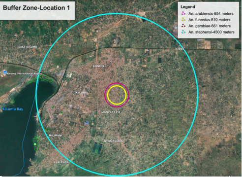
2.8. Vector Host Population Buffer Zones

Download: Download full-size image

Figure 3. An. stephensi flight distance measurements.

Download: Download full-size image

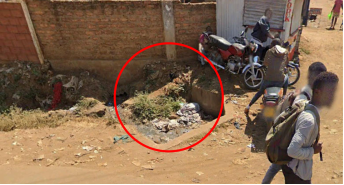
Figure 4. Potential An. stephensi habitat.

3. Results

A Poisson probability regression model was determined by a 95% confidence level, which was employed to ascertain whether the proportions of stratified, sampled An. stephensi's habitat, capture point, estimator determinants differed by sub-county-level model predictions. We considered inference, hypothesis testing, and modeling causal relationships amongst the larval An. stephensi's habitat sampled estimator determinants. The regression analyses assumed independent counts (i.e., n_i), taken at the georeferenced county locations i = 1, 2... n, where each of the regressed discrete integer values was from a Poisson distribution. These counts were described by a set of explanatory variables denoted by matrix X_i, a 1×p vector of estimator determinants for a sampled capture point sub-county geolocation i. The expected value of these data was given by

Mi (X_{i}) = Ni (X_{i}) \exp (X_{i} β),

where the vector of non-redundant parameters was the Poisson rates parameter which was given by

Λ i (X_{i}) = μ_{i} (X_{i}) / Ni (X_{i})

. The rates parameter λ_i(X_i) was both the mean and the variance of the Poisson distribution, whereby each stratified, sampled, sub-county-level entomological estimator determinant was denoted as i. The dependent variable was the prevalence of malaria mortality rates in Kisumu in the regression model. The analysis was performed in R. The sampled data were log-transformed before analyses to normalize the distribution and minimize standard error. All of the covariate estimates for the model were tested using a backward stepwise regression. The most significant predictor was children.

Table 2. Output Summary Poisson Table.

Coefficients	Estimate	Standard Deviation Error	Z Value	Pr (>\|z\|)
Intercept	-2.121858	1.509615	-1.412	0.158
Children <5	-0.001897	0.001801	-1.054	0.292

A spectral signature capture point was performed in PySAL using the georeferenced, stratified regressed capture point, larval, An. stephensi habitat stratified, estimator determinants. An analogous variant of conventional correlation is serial correlation, which pertains to the correlation between values for observations of a single variable, according to some delivery of those values (14). Each georeferenced capture point location became a feature vector containing predictors such as population density and demographic characteristics. The response variable represented a composite larval, An. stephensi habitat exposure index. Geographic coordinates of the centroid were included so spatial patterns could be learned implicitly by the models or explicitly augmented with spatial lag features (e.g., neighboring capture point sentinel site averages).

Using Random Forest, Gradient Boosting, and XGBoost models, we trained supervised learning algorithms to map the relationship between predictor variables and malaria-related outcomes across Kisumu County. This created a structured dataset suitable for comparative machine-learning-based spatial risk prediction.

Table 3. Summary Statistics of Covariates.

Variable	Mean	Std. Dev.	Min	Max
Distance to Water (m)	248.5	198.4	10	850
Elevation (m)	1152.3	18.7	1120	1185
Land Surface Temp (°C)	29.8	2.1	25.8	34.5
Rainfall (mm)	118.4	34.6	60	180
Population Density (persons/km²)	1035	412	280	2150
Built-up Index	0.56	0.18	0.22	0.89

Table 4. Variable Importance from Random Forest Model.

Rank	Predictor Variable	Importance Score
1	Distance to Water	0.241
2	Land Surface Temperature	0.212
3	Built-up Index	0.176
4	Rainfall	0.141
5	Population Density	0.074
6	Elevation	0.041

Table 5. Variable Importance from XGBoost.

Rank	Predictor Variable	Gain (%)
1	Distance to Water	24.8
2	Built-up Index	20.5
3	Land Surface Temperature	18.7
4	Rainfall	14.9
5	Population Density	7.1
6	Elevation	3.2

Table 6. Model Performance Comparison.

Model	Accuracy	Precision	Recall	F1-Score	AUC-ROC
Random Forest	0.86	0.84	0.82	0.83	0.91
Gradient Boosting	0.88	0.86	0.85	0.85	0.93
XGBoost	0.91	0.89	0.88	0.89	0.96

Table 7. Habitat Suitability Prediction by XGBoost.

Habitat ID	Predicted Probability	Predicted Class
H001	0.92	Suitable
H002	0.18	Unsuitable
H003	0.87	Suitable
H004	0.09	Unsuitable
H005	0.95	Suitable
H006	0.31	Unsuitable

The machine learning models identified proximity to water bodies, land surface temperature, urbanization level (built-up index), and rainfall as the strongest determinants of Anopheles stephensi larval habitat occurrence. Among the evaluated algorithms, XGBoost achieved the highest predictive performance (AUC = 0.96), demonstrating superior ability to quantify complex nonlinear relationships and interactions among environmental and anthropogenic predictors. These findings suggest that urban water sources and warm, densely populated environments may provide favorable conditions for An. stephensi establishment across Kisumu County,

During training, the entomological dataset was divided into training and validation sets, allowing the model to learn complex anthropogenic interactions among estimator determinants such as socioeconomic and sociodemographic conditions. Once predicted risk values were quantified spatial statistical techniques were applied to detect hotspot and cold-spot clusters of An. stephensi larval habitats. Predicted capture point habitat risk surfaces were mapped using Python and analyzed with spatial autocorrelation metrics such as Local Moran’s I and Getis-Ord Gi*, which identified statistically significant clusters of high predicted stratified, An. stephensi habitat (hotspots) and low predicted risk (cold spots). Our assumption was that in large metropolitan areas such as downtown urban Kisumu, stratified clusters may correspond to patterns in breeding sites, transportation distribution networks, socioeconomic vulnerability, or service access gaps. The machine-learning predictions combined with spatial clustering produced a county-wide geospatial An. stephensi's habitat map is related to transmission-related risks concentrated geographically.

Afterwards, neighboring georeferenced, sub-county-level larval An. stephensi habitat stratified, capture point, hot and cold spots were identified based on the stratified, measured, epidemiological and entomological sampled, non-time series, dependent discrete integer values, in an n-by-n binary geographic connectivity/weights matrix, C (Equation (33)).

\frac{\begin{matrix} n \\ \sum \\ i = 1 \end{matrix} (x_{i} - \overset{̅}{x}) (y_{i} - \overset{̅}{y}) / n}{\sqrt{\begin{matrix} n \\ \sum \\ i = 1 \end{matrix} {(x_{i} - \overset{̅}{x})}^{2} / n} \sqrt{\begin{matrix} n \\ \sum \\ i = 1 \end{matrix} {(y_{i} - \overset{̅}{y})}^{2} / n}}

(33)

Thereafter, eigen-autocorrelation residual coefficients were expressible in terms of the product moment correlation coefficient formula. However, with neighboring capture point values y replacing the value of each sampled variable x (33) became:

\frac{\begin{matrix} n \\ \sum \\ i = 1 \end{matrix} (y_{i} - \overset{̅}{y}) \begin{matrix} n \\ \sum \\ j = 1 \end{matrix} c_{ij} (y_{i} - \overset{̅}{y}) / \begin{matrix} n \\ \sum \\ i = 1 \end{matrix} \begin{matrix} n \\ \sum \\ j = 1 \end{matrix} c_{ij}}{\sqrt{\begin{matrix} n \\ \sum \\ i = 1 \end{matrix} {(y_{i} - \overset{̅}{y})}^{2} / n} \sqrt{\begin{matrix} n \\ \sum \\ i = 1 \end{matrix} {(y_{i} - \overset{̅}{y})}^{2}} / n}

(34)

The left-hand expression converted to the right side in the stratified, eigen-autocorrelation, habitat, spectral signature, model, by substituting the numerator term only when a 1 appeared in the matrix C and by averaging the numerator cross-product terms over the total number of sampled estimator determinants, denoted in matrix C, i.e.

\sum_{i = 1}^{n} \sum_{j - 1}^{n} C_{ij}

. The denominator of the revised expression of Equation (33) was the sample variance of Y,

s_{Y}^{2}

. Coupling this with part of the accompanying numerator term rendered

(y_{i} - \overset{̅}{y}) / s_{Y} \sum_{j = 1}^{n} c_{ij} (y_{i} - \overset{̅}{y}) / s_{Y} = z_{Y, i} \sum_{i = 1}^{n} c_{ij} z_{Y, j}

(35)

Standard normal deviate (i.e. z score) notation

z_{y}

was calculable. The right-hand expression of Equation (33) was Moran’s coefficient. The coefficient resembled a Pearson product-moment correlation coefficient, ranging in value from −1 to +1. As indicated by −(n − 1)/n, Moran’s was influenced by a distribution of a number of georeferenced, stratified, neighbors (via

\sum_{j = 1}^{n} C_{ij}

and via

{(y_{i} - \overset{̅}{y})}^{2} / s_{y}^{2} = Z_{{Y,}_{i}} \times Z_{Y_{j}}

. A standard bivariate regression included an intercept regression of

\sum_{j = 1}^{n} C_{ij}

on Zy.

Download: Download full-size image

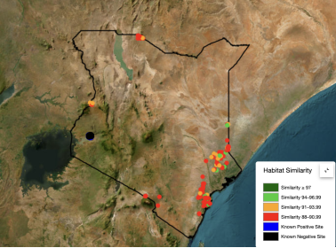
Figure 5. Potential Hot & Cold spots of Anopheles Stephensi habitats in Kenya.

A Box-Cox type of power transformation was subsequently employed for normal approximation analysis purposes, so that the frequency distributions of the georeferenced, sampled, capture point, larval An. stephensi's habitat estimator determinants approximated a bell-shaped curve. The eigen-spatial filter construction methodology transformation procedure was used, as proposed by

[15]

, which depends on the eigenfunctions of matrix (I−11^T/n)C(I−11^T/n), where I denoted the identity matrix, 1 was an n-by-1 vector of ones, and T denoted matrix transpose, a term which appeared in the numerator of Moran’s Coefficient. According to

[15]

, the first eigenvector, E₁, is the set of numerical values with the largest spatial indices achievable by any set for the spatial arrangement defined by the connectivity matrix C. The second eigenvector is the set of values with the largest achievable autocorrelated values by any set that is uncorrelated with E₁. The third eigenvector is the third such set of values, and so on. This sequential construction of eigenvectors continued in the stratified, capture point, An. stephensi habitat prognosticative model through E_n, where the set of measured stratified, eigen-autocorrelated, An. stephensi, habitat estimator determinant, with the largest positive to negative capture point values, was rendered. Moran’s Coefficient was achieved by the set uncorrelated with the preceding (n − 1) eigenvectors.

To identify the stratified geospatial larval An. stephensi habitat clusters that could be uncovered with eigen-spatial filtering, Thiessen polygon surface partitions were generated to construct geographic neighbor matrices in PySAL, whereby each hot and cold spot in Kisumu County was denoted by matrix C. Entries in matrix C were 1 if two An. stephensi habitat sampled, georeferenced, capture points shared a common Thiessen polygon boundary and 0 otherwise. The diagonal was coded 0. Next, the linkage structure for each surface was edited to remove unlikely geographic neighbors to identify pairs of georeferenceable capture point locations sharing a common Thiessen polygon boundary. Eigenvectors of a modified version of this matrix C furnished synthetic variates that constituted distinct habitat map patterns representing the full range of non-zero, Gaussian, eigen-autocorrelated possibilities. Attention was restricted to those map patterns associated with at least a minimum level of eigenized autocorrelation statistics, which, for implementation purposes here, was definable by Moran’s Coefficient using max > 0.25. Moran’s Coefficient denoted the j^th value, and Moran’s Coefficient, max_x, the maximum value of the eigen-autocorrelation index. This threshold value allowed two candidate sets of eigenvectors to be considered for substantial positive and substantial negative eigen-autocorrelation, respectively.

We performed the Moran’s coefficient decomposition to quantitate whether or not equation (33) can be replaced by:

P (Yi = 1 | Ei, K) = \exp (α + Ei, Kβ) / [1 + \exp (α + Ei, Kβ)]

(36)

This was determined by K denoting some subset of the n eigenvectors derived from the eigen-spatial filter eigen-decomposition analyses of the remotely entomologically sampled, georeferenced, stratified, capture point, An. stephensi's habitat estimator determinants were chosen by the supervised selection criteria. The

E_{i, K}

was an n-by-K matrix whose columns were the K selected eigenvectors. This allowed dispensing with the

P \sum_{j = 1}^{n} C_{ij} Y_{j}

term by shifting spatial dependence effects to the large-scale variation term represented by E_i,Kβ, forcing ρ to 0 in the eigen-autocorrelation capture point model. We let α_i be the constant α. Only the stratified covariates were included in the habitat model specification. A link between Equations (33) and (34) was gleaned from the following algebraic manipulations:

P (Y = 1| CY) = P (Y = 1| E Λ ETY) = P (Y = 1| Eδ),

where Λ was a diagonal matrix of eigenvalues whose order was the same as the corresponding eigenvectors in matrix E, δ was a vector of coefficients where superscript T denoted the matrix transpose. A straightforward extension of Equation (34) included the sub- county-level, stratified, An. stephensi habitat estimator determinant model specification; the version selected focused on the eigenvector eigen-spatial filter. The parameters α and β in Equation (34) were subsequently estimated with the method of maximum likelihood.

The Moran scatter plot was also employed for the visualization of the zero/non-zero residual eigen-autocorrelation in the sub-county-level empirical, sampled georeferenced entomological datasets. The Moran's scatterplot was based upon Equation (36), as was a plot of the pairs (

(y_{i} - \overset{̅}{y}) / s_{Y}, \sum_{j = 1}^{n} C_{ij} (y_{i} - \overset{̅}{y}) / s_{Y})

, linking it directly to standard correlation and regression analyses of the larval sampled An. stephensi habitat estimator determinants. To construct the scatter plot, the count values of the stratified entomological data, Y, were converted to z scores. Next, those adjacent or nearby georeferenced sub-county-level z-score values of Y were summed using the matrix product Czy, where Zy was the vector concatenation of the individual Zy values. Finally, the coordinates of the sampled CC estimator determinants were quantified in eigenvector eigen-geospace. We noted that

Z_{Y, i}, \sum_{j = 1}^{n} C_{ij} Z_{Y, j}

), i= 1, 2, n, was plottable on the graph, where the vertical axis was Czy and the horizontal axis was Zy. Significant hot spots (p < 0.01) were concentrated in Kisumu, characterized by higher socioeconomic deprivation and lower screening coverage. In contrast, statistically significant cold spots (p < 0.01) were observed in the entomological intervention site corresponding to areas with higher socioeconomic status and greater access to preventive services.

The vertical axis point was written in the stratified, capture point, larval An. stephensi's habitat model as

\sum_{j = 1}^{n} w_{ij} (y_{i} - \overset{̅}{y}) / s_{Y}

, where

w_{ij} = c_{ij} / \sum_{j = 1}^{n} c_{ij}

resulting in an averaging of the surrounding nearby habitat sampled count values (y_j − ȳ)/s_Y for each capture point i's using (y_i − ȳ)/s_Y. The quantities

\sum_{j = 1}^{n} c_{ij} (y_{j} - \overset{̅}{y}) / s_{Y}

were employed as the slope of the regression line for Moran's scatterplot, which in this experiment was the unstandardized Moran’s coefficient. The w_ij values were organized in an n-by-n matrix w, which was the row-standardized counterpart to matrix C. Finally, the coordinate pairs

Z_{Y, i}, \sum_{j = 1}^{n} c_{ij} z_{Y, j}

i= 1, 2, n, were plotted on the graph where the vertical axis was CZY and the horizontal axis was Zy. The unstandardized Moran’s coefficient was computed using the standard bivariate regression technique Czy on Zy, yielding bcy/y while specifying a non-intercept option. A no-intercept regression of C1 provided the discrete integer value for each, producing the standardization coefficient b_c_1/1− Moran coefficient =b_cy_/_y/b_c_1/1.

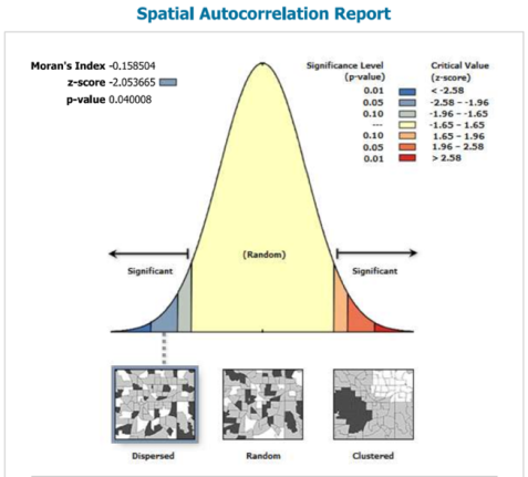
Table 8. Global Moran’s I.

Statistic	Value
Moran’s Index	-0.158504
Expected Index	-0.018519
Variance	0.004646
z-score	-2.053665
p-value	0.040008

Download: Download full-size image

Figure 6. Eigen-spatial Autocorrelation Report.

4. Discussion

A Poisson regression model is well-suited for analyzing county-level, stratifiable An. stephensi's habitat count data, such as the number of cases, because it explicitly models non-negative integer outcomes while accounting for differing population sizes. In this framework, the expected count in each sampled capture point in Kisumu was modeled as a function of covariates (e.g., median income, LULC composition, etc.) through a log link function. To properly adjust for variation in population at risk, an offset term, the log of the children < 5 population at risk in each capture point, was included, allowing the model to estimate incidence rate ratios rather than raw counts. Covariates were evaluated based on statistical significance, effect size (incidence rate ratios), model fit criteria (e.g., AIC), and potential confounding or collinearity. Since overdispersion was present (variance exceeding the mean), a negative binomial extension was employed to ensure valid inference. This approach enabled the identification of statistically meaningful An. stephensi habitat predictors associated with higher or lower incidence across sampled capture points.

County-wide geospatial prediction of An. stephensi habitat and transmission-related hotspot and cold-spot clusters in Kisumu can be derived from capture points by aggregating seasonal estimator determinants and using those variables as predictors in machine-learning models such as Random Forest, Gradient Boosting, and XGBoost. Each georeferenced, stratified capture point acts as a spatial observation with demographic, health, and geographic features, allowing a sub-county level An. stephensi's larval habitat model to learn nonlinear relationships between local conditions.

XGBoost iteratively improved prediction accuracy by correcting previous An. stephensi's habitat model errors and optimizing performance with regularization and efficient tree construction. The resulting predicted malaria prevalence rates scores for every georeferenced capture point was mapped and analyzed with algorithmic clustering techniques to identify statistically significant hotspots (high-risk areas) and cold spots (low-risk areas). This produced a county-wide geospatial risk probability raster surface larval An. stephensi habitats. We were able to target interventions in high-risk regions such as major metropolitan areas in Kisumu.

Summary diagnostics from the second-order eigenfunction eigen-decomposition algorithm revealed capture points with high positive eigenvector values, which we interpreted as related to high usage and transaction incidence [i.e., potential hot spots]. Capture points with strongly negative values and low rates represented cold spots. Furthermore, because eigenfunctions extract structured eigenized spatial autocorrelation coefficients rather than random estimator determinant variation

[14]

, these models can help distinguish meaningful geographic clustering from noise, leading to a more stable and statistically grounded identification of localized high and low-risk An. stephensi habitat -related sub-county level, georeferenceable capture point, signature, interpolated areas.

Second-order eigenfunction decomposition can be used to uncover meaningful spatial patterns in malaria risk by analyzing geographic data such as rainfall, temperature, land cover, and standing-water distribution. In this experiment, spatial relationships between An. stephensi's habitat capture point locations were represented in a matrix, and the second-order eigenfunctions captured the dominant modes of variation after the primary trend was removed. These eigenfunctions highlighted geographic disparities, such as clusters of wetlands, irrigation zones, or poorly drained urban areas, where environmental conditions were most conducive to mosquito breeding. By linking these spatial modes to surveillance data on the malaria vector, particularly species like An. stephensi, public-health planners can map high-priority larval habitats with greater precision. The resulting spatial insights can support targeted interventions such as S&D-LSM in Kisumu County, such as draining stagnant water, environmental modification, or localized larvicide application, allowing resources to be concentrated in the areas where they will have the greatest impact on reducing mosquito populations and interrupting malaria transmission.

By integrating statistical modeling, satellite-based spectral analysis, and machine learning spatial forecasting, can demonstrate a novel approach for scaling localized S&D-LSM from Kisumu County activity patterns to a broader full country-wide geographic context. The resulting Country-wide risk maps can provide a data-driven framework for identifying priority areas for intervention and for improving the spatial targeting of public health resources aimed at addressing the ongoing malaria crisis in Kenya.

Future research should also incorporate Exponential Generalized Autoregressive Conditional Heteroskedasticity (EGARCH) models to investigate the temporal dynamics and volatility of An. stephensi habitat suitability and malaria transmission risk across Kenya. While spatial eigen-decomposition approaches can identify geographic clustering and spatial disparities in vector habitats, EGARCH models may provide a framework for examining time-varying variability and asymmetric responses in environmental and epidemiological time series.

Unlike conventional time-series models that assume constant variance, EGARCH may explicitly model conditional heteroscedasticity, allowing fluctuations in malaria incidence, larval habitat abundance, rainfall, temperature, humidity, and vegetation indices to exhibit periods of high and low volatility. The logarithmic variance specification of EGARCH may ensure positive variance estimates without imposing non-negativity constraints and enable the detection of asymmetric effects, whereby unusually wet or dry seasons may have differing impacts on vector proliferation and disease risk.

5. Conclusion

In conclusion, an integrated methodological remote sensing and machine learning approach can enable 10-m resolution spectral signatures associated with An. stephensi stratified larval habitats at the capture point level to be generalized and spatially scaled up to the county-wide level. Eigen-decomposition of a spatial weights matrix can help identify noisy non-Gaussian outliers in georeferenceable An. stephensi stratified hot and cold spots interpolated from a georeferenced breeding site capture point. The algorithm can isolate a structured spatial pattern that can represent clustering contrast in eigenvector eigen-geospace. When decomposing a spatial weight matrix encoded with georeferenced capture point An. stephensi larval habitat sampled estimator determinants as neighbors at the sub-county level the eigenvectors generated can delineate independent spatial patterns which can be embedded in the geography. In this experiment, these patterns reflected regional groupings of georeferenced capture points that shared similar An. stephensi related risk probability level throughout Kisumu. These predictive sub-county-level maps can identify potential clusters of An. stephensi, larval habitat with a potentially elevated risk of malaria transmission for determining a potential intervention site for implementing S&D-LSM.

Abbreviations

An. stephensi	Anopheles Stephensi
DDT	dichlorodiphenyltrichloroethane
d. f.	Degrees of Freedom
GLMM	Generalized Linear Mixed Model
IR	Infrared
IRS	Indoor Residual Spraying
LLINs	Long-lasting Insecticidal Nets
LSM	Larval Source Management
LULC	Land Use Land Cover
MLE	Maximum Likelihood Estimation
PDF	Probability Density Function
S&D-LSM	“Seek and Destroy” Larval Source Management
XGBoost	Extreme Gradient Boosting

Author Contributions

Odelia Asher: Conceptualization, Data curation, Investigation, Writing – original draft

Rishil Shah: Formal Analysis, Methodology, Software, Visualization, Writing – review & editing

Aarya Satardekar: Investigation, Validation, Writing – review & editing

Anusha Parajuli: Investigation, Validation, Writing – review & editing

Namit Choudhari: Methodology, Visualization, Writing – review & editing

James Jedrzejczyk: Resources, Validation, Writing – review & editing

Joseph Mwangangi: Investigation, Resources, Writing – review & editing

Charles Mbogo: Resources, Supervision, Writing – review & editing

Benjamin Jacob: Conceptualization, Formal Analysis, Methodology, Supervision, Writing – review & editing

Conflicts of Interest

The authors declare no conflicts of interest.

References

[1]	Tuteja, R. (2007). Malaria – An Overview. The FEBS Journal, 274(18), 4670-4679. https://doi.org/10.1111/j.1742-4658.2007.05997.x
[2]	Severe Malaria Observatory. (n.d.). Kenya: Malaria facts. https://www.severemalaria.org/countries/kenya
[3]	Nicholas, K., Bernard, G., Bryson, N., Mukabane, K., Kilongosi, M., Ayuya, S., Mulama, D. H. (2021). Abundance and distribution of malaria vectors in various aquatic habitats and land use types in Kakamega County, highlands of Western Kenya. Ethiopian Journal of Health Sciences, 31 (2), 247-256. https://doi.org/10.4314/ejhs.v31i2.7
[4]	Taylor, R., Messenger, L, A., Abeku, T, A., Clarke, S, E., Yadav, R. S., & Lines, J. (2024). Invasive Anopheles Stephensi in Africa: Insights from Asia. Trends in Parasitology, 40(8), 731-743. https://doi.org/10.1016/j.pt.2024.06.008
[5]	Ochomo, E. O., Milanoi, S., Abong'o, B., Onyango, B., Muchoki, M., Omoke, D., Olanga, E., Njoroge, L., Juma, E. O., Otieno, J. D., Matoke-Muhia, D., Kamau, L., Rafferty, C., Gimnig, J. E., Shieshia, M., Wacira, D., Mwangangi, J., Maia, M., Chege, C., Omar, A., … Kariuki, L. (2023). Detection of Anopheles Stephensi Mosquitoes by Molecular Surveillance, Kenya. Emerging infectious diseases, 29(12), 2498–2508. https://doi.org/10.3201/eid2912.230637
[6]	Dube, M. V., & Gakhar, S. K. (2010). Genetic differentiation between three ecological variants (‘type’, ‘mysorensis’ and ‘intermediate’) of malaria vector Anopheles Stephensi (Diptera: Culicidae). Insect Science, 17(4), 335-343. https://doi.org/10.1111/j.1744-7917.2010.01316.x
[7]	Zhou, G., Zhong, D., Yewhalaw, D., & Yan, G. (2024). Anopheles Stephensi ecology and control in Africa. Trends in parasitology, 40(2), 102–105. https://doi.org/10.1016/j.pt.2023.11.011
[8]	Otambo, W. O., Onyango, P. O., Wang, C., Olumeh, J., Ondeto, B. M., Lee, M. C., Atieli, H., Githeko, A. K., Kazura, J., Zhong, D., Zhou, G., Githure, J., Ouma, C., & Yan, G. Influence of Landscape Heterogeneity on Entomological and Parasitological Indices of Malaria in Kisumu, Western Kenya. Parasites & Vectors. 2022, 15(1), 340. https://doi.org/10.1186/s13071-022-05447-9
[9]	Machani, M. G., Onyango, S. A., Nzioki, I., Milanoi, S., Nattoh, G., Githure, J., Atieli, H., Wang, C., Lee, M., Zhou, G., Githeko, A., Afrane, Y. A., Ochomo, E., & Yan, G. (2024). Bionomics and distribution of malaria vectors in Kisumu city, Western Kenya: Implications for urban malaria transmission. Research Square. https://doi.org/10.21203/rs.3.rs-4943539/v1
[10]	Wikipedia. Kisumu. Available from: https://en.wikipedia.org/wiki/Kisumu (accessed 21 April 2026).
[11]	Teshome, A., Erko, B., Golassa, L. et al. Resistance of Anopheles stephensi to selected insecticides used for indoor residual spraying and long-lasting insecticidal nets in Ethiopia. Malar J 22, 218 (2023). https://doi.org/10.1186/s12936-023-04649-5
[12]	Hosmer, D. W., Lemeshow, S. Applied Logistic Regression. 2^nd Edition. New York, NY: John Wiley & Sons, Inc; 2000. https://doi.org/10.1002/0471722146
[13]	Greenwood, P. E. and Nikulin, M. S. A Guide to Chi-Squared Testing. 1^st Edition. New York, NY: John Wiley & Sons, 1996.
[14]	Griffith, 2003 Griffith, D. A. Spatial Autocorrelation and Spatial Filtering: Gaining Understanding Through Theory and Scientific Visualization. 1^st Edition. New York, NY: Springer-Verlag Berlin Heidelberg; 2023. https://doi.org/10.1007/978-3-540-24806-4
[15]	Jacob, B. G., Izureta, R., Bell, J., Parikh, J., Louh, D., Gates, T., Murray, K., White, L., and Aceng, J. R. Approximating Non-Asymptoticalness, Skew Heterr (2023). https://doi.org/10.5923/j.ajms.20231301.01

Cite This Article

Plain Text BibTeX RIS

APA Style

Asher, O., Shah, R., Satardekar, A., Parajuli, A., Choudhari, N., et al. (2026). Scaling Point-Based Habitat Observations of Anopheles stephensi Using XGBoost to Support Seek-and-Destroy Larval Source Management in Kisumu, Kenya. American Journal of Entomology, 10(3), 45-61. https://doi.org/10.11648/j.aje.20261003.11

Copy | Download

ACS Style

Asher, O.; Shah, R.; Satardekar, A.; Parajuli, A.; Choudhari, N., et al. Scaling Point-Based Habitat Observations of Anopheles stephensi Using XGBoost to Support Seek-and-Destroy Larval Source Management in Kisumu, Kenya. Am. J. Entomol. 2026, 10(3), 45-61. doi: 10.11648/j.aje.20261003.11

Copy | Download

AMA Style

Asher O, Shah R, Satardekar A, Parajuli A, Choudhari N, et al. Scaling Point-Based Habitat Observations of Anopheles stephensi Using XGBoost to Support Seek-and-Destroy Larval Source Management in Kisumu, Kenya. Am J Entomol. 2026;10(3):45-61. doi: 10.11648/j.aje.20261003.11

Copy | Download

@article{10.11648/j.aje.20261003.11,
  author = {Odelia Asher and Rishil Shah and Aarya Satardekar and Anusha Parajuli and Namit Choudhari and James Jedrzejczyk and Joseph Mwangangi and Charles Mbogo and Benjamin Jacob},
  title = {Scaling Point-Based Habitat Observations of Anopheles stephensi Using XGBoost to Support Seek-and-Destroy Larval Source Management in Kisumu, Kenya},
  journal = {American Journal of Entomology},
  volume = {10},
  number = {3},
  pages = {45-61},
  doi = {10.11648/j.aje.20261003.11},
  url = {https://doi.org/10.11648/j.aje.20261003.11},
  eprint = {https://article.sciencepublishinggroup.com/pdf/10.11648.j.aje.20261003.11},
  abstract = {The invasive malaria vector Anopheles stephensi poses an emerging challenge to malaria control in rapidly urbanizing regions of East Africa. This study evaluates the spatial distribution and potential spread of An. stephensi across Kisumu County by integrating field entomological observations with machine learning models applied to satellite-derived environmental data. The primary objective was to scale habitat signatures identified at confirmed georeferenced capture locations to the county level to support a targeted “Seek-and-Destroy” larval source management (S&D-LSM) strategy. Confirmed larval and adult capture points were used to extract environmental predictors from 10-m resolution visible and near-infrared (IR) bands derived from Sentinel-2 imagery. These spectral variables, along with derived indices representing vegetation structure, surface moisture, and urban disturbance, served as input features for predictive modeling. Three ensemble machine learning approaches—Random Forest, Gradient Boosting, and Extreme Gradient Boosting (XGBoost)—were implemented to model the relationship between environmental signatures and observed mosquito presence. Each model was trained using capture locations and background samples to classify potential breeding habitats across the landscape. Model performance was evaluated using cross-validation and standard classification metrics, and the resulting predictions were used to generate habitat suitability maps for the entirety of Kisumu County. Ensemble tree methods effectively captured nonlinear relationships between spectral features and mosquito habitat conditions, enabling the identification of spatial clusters of high-probability breeding environments. XGBoost achieved the highest predictive performance (AUC = 0.96), demonstrating superior ability to quantify complex nonlinear relationships and interactions among environmental and anthropogenic An. stephensi predictors. The eigen-autocorrelation statistics revealed a Moran’s Index of -0.159, a variance of 0.005, a z-score of 0.019 and a p-value of 0.04. Areas of elevated suitability were frequently associated with dense settlement patterns, infrastructure corridors, and locations with intermittent water storage or container habitats. The resulting risk surfaces enabled vector control teams to prioritize surveillance and intervention efforts. By spatially targeting activities toward high-probability sites, the program operationalized an S&D-LSM approach focused on rapid detection and elimination of breeding habitats. This study demonstrates that integrating remote sensing with ensemble machine learning provides a scalable framework for monitoring invasive malaria vectors and supporting targeted urban malaria control interventions.},
 year = {2026}
}

Copy | Download

TY  - JOUR
T1  - Scaling Point-Based Habitat Observations of Anopheles stephensi Using XGBoost to Support Seek-and-Destroy Larval Source Management in Kisumu, Kenya
AU  - Odelia Asher
AU  - Rishil Shah
AU  - Aarya Satardekar
AU  - Anusha Parajuli
AU  - Namit Choudhari
AU  - James Jedrzejczyk
AU  - Joseph Mwangangi
AU  - Charles Mbogo
AU  - Benjamin Jacob
Y1  - 2026/08/06
PY  - 2026
N1  - https://doi.org/10.11648/j.aje.20261003.11
DO  - 10.11648/j.aje.20261003.11
T2  - American Journal of Entomology
JF  - American Journal of Entomology
JO  - American Journal of Entomology
SP  - 45
EP  - 61
PB  - Science Publishing Group
SN  - 2640-0537
UR  - https://doi.org/10.11648/j.aje.20261003.11
AB  - The invasive malaria vector Anopheles stephensi poses an emerging challenge to malaria control in rapidly urbanizing regions of East Africa. This study evaluates the spatial distribution and potential spread of An. stephensi across Kisumu County by integrating field entomological observations with machine learning models applied to satellite-derived environmental data. The primary objective was to scale habitat signatures identified at confirmed georeferenced capture locations to the county level to support a targeted “Seek-and-Destroy” larval source management (S&D-LSM) strategy. Confirmed larval and adult capture points were used to extract environmental predictors from 10-m resolution visible and near-infrared (IR) bands derived from Sentinel-2 imagery. These spectral variables, along with derived indices representing vegetation structure, surface moisture, and urban disturbance, served as input features for predictive modeling. Three ensemble machine learning approaches—Random Forest, Gradient Boosting, and Extreme Gradient Boosting (XGBoost)—were implemented to model the relationship between environmental signatures and observed mosquito presence. Each model was trained using capture locations and background samples to classify potential breeding habitats across the landscape. Model performance was evaluated using cross-validation and standard classification metrics, and the resulting predictions were used to generate habitat suitability maps for the entirety of Kisumu County. Ensemble tree methods effectively captured nonlinear relationships between spectral features and mosquito habitat conditions, enabling the identification of spatial clusters of high-probability breeding environments. XGBoost achieved the highest predictive performance (AUC = 0.96), demonstrating superior ability to quantify complex nonlinear relationships and interactions among environmental and anthropogenic An. stephensi predictors. The eigen-autocorrelation statistics revealed a Moran’s Index of -0.159, a variance of 0.005, a z-score of 0.019 and a p-value of 0.04. Areas of elevated suitability were frequently associated with dense settlement patterns, infrastructure corridors, and locations with intermittent water storage or container habitats. The resulting risk surfaces enabled vector control teams to prioritize surveillance and intervention efforts. By spatially targeting activities toward high-probability sites, the program operationalized an S&D-LSM approach focused on rapid detection and elimination of breeding habitats. This study demonstrates that integrating remote sensing with ensemble machine learning provides a scalable framework for monitoring invasive malaria vectors and supporting targeted urban malaria control interventions.
VL  - 10
IS  - 3
ER  -

Copy | Download

Author Information

Odelia Asher

College of Public Health, University of South Florida, Tampa, USA

Research Fields: Medical Entomology, Vector Ecology, Malaria Control, Public Health, Spatial Epidemiology.

Contact Email
Rishil Shah

Bellini College of Artificial Intelligence, Cybersecurity and Computing, University of South Florida, Tampa, USA

Research Fields: Artificial Intelligence, Machine Learning, Geospatial Analytics, Remote Sensing, Spatial Modeling.

Contact Email
Aarya Satardekar

Department of Health Policy and Systems Management, University of South Florida, Tampa, USA

Research Fields: Health Policy, Health Systems Management, Public Health, Epidemiology, Healthcare Research.

Contact Email
Anusha Parajuli

Department of Epidemiology, University of South Florida, Tampa, USA

Research Fields: Epidemiology, Infectious Diseases, Public Health, Disease Surveillance, Statistical Analysis.

Contact Email
Namit Choudhari

School of Geosciences, University of South Florida, Tampa, USA

Research Fields: Remote Sensing, Geographic Information Systems, Spatial Analysis, Environmental Modeling, Geospatial Science.

Contact Email
James Jedrzejczyk

College of Public Health, University of South Florida, Tampa, USA

Research Fields: Public Health, Global Health, Vector Surveillance, Environmental Health, Research Methodology.

Contact Email
Joseph Mwangangi

Centre for Geographic Medicine Research, Kenya Medical Research Institute, Mombasa, Kenya

Research Fields: Medical Entomology, Vector Control, Malaria Surveillance, Tropical Diseases, Public Health.

Contact Email
Charles Mbogo

Wellcome Trust Research Programme, Kenya Medical Research Institute, Kilifi, Kenya

Research Fields: Medical Entomology, Malaria Control, Vector Biology, Tropical Medicine, Disease Prevention.

Contact Email
Benjamin Jacob

Department of Biostatistics and Data Science, University of South Florida, Tampa, USA

Research Fields: Biostatistics, Data Science, Machine Learning, Spatial Statistics, Public Health Analytics.

Contact Email

Download PDF

Submit an Article

Plain Text BibTeX RIS

APA Style

Asher, O., Shah, R., Satardekar, A., Parajuli, A., Choudhari, N., et al. (2026). Scaling Point-Based Habitat Observations of Anopheles stephensi Using XGBoost to Support Seek-and-Destroy Larval Source Management in Kisumu, Kenya. American Journal of Entomology, 10(3), 45-61. https://doi.org/10.11648/j.aje.20261003.11

Copy | Download

ACS Style

Asher, O.; Shah, R.; Satardekar, A.; Parajuli, A.; Choudhari, N., et al. Scaling Point-Based Habitat Observations of Anopheles stephensi Using XGBoost to Support Seek-and-Destroy Larval Source Management in Kisumu, Kenya. Am. J. Entomol. 2026, 10(3), 45-61. doi: 10.11648/j.aje.20261003.11

Copy | Download

AMA Style

Asher O, Shah R, Satardekar A, Parajuli A, Choudhari N, et al. Scaling Point-Based Habitat Observations of Anopheles stephensi Using XGBoost to Support Seek-and-Destroy Larval Source Management in Kisumu, Kenya. Am J Entomol. 2026;10(3):45-61. doi: 10.11648/j.aje.20261003.11

Copy | Download

@article{10.11648/j.aje.20261003.11,
  author = {Odelia Asher and Rishil Shah and Aarya Satardekar and Anusha Parajuli and Namit Choudhari and James Jedrzejczyk and Joseph Mwangangi and Charles Mbogo and Benjamin Jacob},
  title = {Scaling Point-Based Habitat Observations of Anopheles stephensi Using XGBoost to Support Seek-and-Destroy Larval Source Management in Kisumu, Kenya},
  journal = {American Journal of Entomology},
  volume = {10},
  number = {3},
  pages = {45-61},
  doi = {10.11648/j.aje.20261003.11},
  url = {https://doi.org/10.11648/j.aje.20261003.11},
  eprint = {https://article.sciencepublishinggroup.com/pdf/10.11648.j.aje.20261003.11},
  abstract = {The invasive malaria vector Anopheles stephensi poses an emerging challenge to malaria control in rapidly urbanizing regions of East Africa. This study evaluates the spatial distribution and potential spread of An. stephensi across Kisumu County by integrating field entomological observations with machine learning models applied to satellite-derived environmental data. The primary objective was to scale habitat signatures identified at confirmed georeferenced capture locations to the county level to support a targeted “Seek-and-Destroy” larval source management (S&D-LSM) strategy. Confirmed larval and adult capture points were used to extract environmental predictors from 10-m resolution visible and near-infrared (IR) bands derived from Sentinel-2 imagery. These spectral variables, along with derived indices representing vegetation structure, surface moisture, and urban disturbance, served as input features for predictive modeling. Three ensemble machine learning approaches—Random Forest, Gradient Boosting, and Extreme Gradient Boosting (XGBoost)—were implemented to model the relationship between environmental signatures and observed mosquito presence. Each model was trained using capture locations and background samples to classify potential breeding habitats across the landscape. Model performance was evaluated using cross-validation and standard classification metrics, and the resulting predictions were used to generate habitat suitability maps for the entirety of Kisumu County. Ensemble tree methods effectively captured nonlinear relationships between spectral features and mosquito habitat conditions, enabling the identification of spatial clusters of high-probability breeding environments. XGBoost achieved the highest predictive performance (AUC = 0.96), demonstrating superior ability to quantify complex nonlinear relationships and interactions among environmental and anthropogenic An. stephensi predictors. The eigen-autocorrelation statistics revealed a Moran’s Index of -0.159, a variance of 0.005, a z-score of 0.019 and a p-value of 0.04. Areas of elevated suitability were frequently associated with dense settlement patterns, infrastructure corridors, and locations with intermittent water storage or container habitats. The resulting risk surfaces enabled vector control teams to prioritize surveillance and intervention efforts. By spatially targeting activities toward high-probability sites, the program operationalized an S&D-LSM approach focused on rapid detection and elimination of breeding habitats. This study demonstrates that integrating remote sensing with ensemble machine learning provides a scalable framework for monitoring invasive malaria vectors and supporting targeted urban malaria control interventions.},
 year = {2026}
}

Copy | Download

TY  - JOUR
T1  - Scaling Point-Based Habitat Observations of Anopheles stephensi Using XGBoost to Support Seek-and-Destroy Larval Source Management in Kisumu, Kenya
AU  - Odelia Asher
AU  - Rishil Shah
AU  - Aarya Satardekar
AU  - Anusha Parajuli
AU  - Namit Choudhari
AU  - James Jedrzejczyk
AU  - Joseph Mwangangi
AU  - Charles Mbogo
AU  - Benjamin Jacob
Y1  - 2026/08/06
PY  - 2026
N1  - https://doi.org/10.11648/j.aje.20261003.11
DO  - 10.11648/j.aje.20261003.11
T2  - American Journal of Entomology
JF  - American Journal of Entomology
JO  - American Journal of Entomology
SP  - 45
EP  - 61
PB  - Science Publishing Group
SN  - 2640-0537
UR  - https://doi.org/10.11648/j.aje.20261003.11
AB  - The invasive malaria vector Anopheles stephensi poses an emerging challenge to malaria control in rapidly urbanizing regions of East Africa. This study evaluates the spatial distribution and potential spread of An. stephensi across Kisumu County by integrating field entomological observations with machine learning models applied to satellite-derived environmental data. The primary objective was to scale habitat signatures identified at confirmed georeferenced capture locations to the county level to support a targeted “Seek-and-Destroy” larval source management (S&D-LSM) strategy. Confirmed larval and adult capture points were used to extract environmental predictors from 10-m resolution visible and near-infrared (IR) bands derived from Sentinel-2 imagery. These spectral variables, along with derived indices representing vegetation structure, surface moisture, and urban disturbance, served as input features for predictive modeling. Three ensemble machine learning approaches—Random Forest, Gradient Boosting, and Extreme Gradient Boosting (XGBoost)—were implemented to model the relationship between environmental signatures and observed mosquito presence. Each model was trained using capture locations and background samples to classify potential breeding habitats across the landscape. Model performance was evaluated using cross-validation and standard classification metrics, and the resulting predictions were used to generate habitat suitability maps for the entirety of Kisumu County. Ensemble tree methods effectively captured nonlinear relationships between spectral features and mosquito habitat conditions, enabling the identification of spatial clusters of high-probability breeding environments. XGBoost achieved the highest predictive performance (AUC = 0.96), demonstrating superior ability to quantify complex nonlinear relationships and interactions among environmental and anthropogenic An. stephensi predictors. The eigen-autocorrelation statistics revealed a Moran’s Index of -0.159, a variance of 0.005, a z-score of 0.019 and a p-value of 0.04. Areas of elevated suitability were frequently associated with dense settlement patterns, infrastructure corridors, and locations with intermittent water storage or container habitats. The resulting risk surfaces enabled vector control teams to prioritize surveillance and intervention efforts. By spatially targeting activities toward high-probability sites, the program operationalized an S&D-LSM approach focused on rapid detection and elimination of breeding habitats. This study demonstrates that integrating remote sensing with ensemble machine learning provides a scalable framework for monitoring invasive malaria vectors and supporting targeted urban malaria control interventions.
VL  - 10
IS  - 3
ER  -

Copy | Download