Abstract
This paper addresses the challenge of uncertainty in reinforcement learning (RL) by presenting a robust policy learning approach based on interval optimization. Traditional RL methods often depend on precise estimations of environment dynamics and reward functions, potentially resulting in sub-optimal or unsafe decisions when faced with real-world ambiguity and limited data. To overcome these limitations, we propose modeling value functions, rewards, and transitions as bounded intervals, thereby explicitly capturing both epistemic uncertainty (arising from incomplete knowledge) and aleatoric uncertainty (stemming from inherent randomness). Our contribution includes formal mathematical frameworks that enable interval-based representation throughout the RL process. We explore strategies for developing policies that are optimized within these interval constraints, ensuring greater resilience to uncertainty and variability. The paper further introduces benchmarking metrics specifically designed to evaluate the effectiveness and robustness of interval-aware RL policies, providing a systematic means of comparison against conventional approaches. To demonstrate the practical value of this methodology, we present a case study focused on financial credit line allocation. The results highlight that interval-aware RL not only enhances safety and reliability in decision-making but also leads to improved outcomes in environments characterized by uncertainty. By moving away from point estimates and adopting interval modeling, our work advocates for a fundamental shift in reinforcement learning practices—enabling more robust, uncertainty-aware policy learning that is well-suited to complex, real-world domains. This approach paves the way for safer and more effective RL deployments across various industries, including finance, healthcare, and robotics.
Keywords
Reinforcement Learning, Deep Learning, Large Language Model, Markov Decision Process
1. Introduction
Reinforcement Learning (RL) is a powerful paradigm for sequential decision-making problems. However, standard RL algorithms assume accurate knowledge of the reward and transition functions or sufficient data to estimate them precisely. In many areas, such as healthcare, finance, or robotics, the environment is either partially observable or exhibits substantial uncertainty.
Interval Optimization in RL addresses this limitation by maintaining bounds on rewards, transition probabilities, and value estimates. Rather than operating on point estimates, it optimizes policies based on worst-case, best-case, or uncertainty-aware criteria.
To address these challenges, the article introduces Interval Optimization as a robust methodology for RL. This approach diverges from traditional models by representing rewards, transitions, and value functions as bounded intervals rather than single-point estimates. By capturing both epistemic uncertainty (stemming from lack of knowledge) and aleatoric uncertainty (arising from randomness in the environment), interval-based RL empowers policy learning that is more resilient to ambiguity. The formal mathematical framework presented in the article lays the foundation for optimizing policies under interval constraints, enabling decision-making that accounts for best-case, worst-case, and uncertainty-aware scenarios.
Benchmarking metrics discussed in the article further reinforce the effectiveness and reliability of interval-aware RL, as demonstrated in the practical case study involving financial credit line allocation. Ultimately, this methodology advocates for an novel approach in RL—moving away from point estimates and towards interval modeling—to enhance safety, robustness, and overall performance in uncertain domains.
Main contributions:
1) The paper introduces a novel interval optimization framework for reinforcement learning, which explicitly models uncertainties by using bounded intervals for rewards, transition probabilities, and value functions.
2) It develops rigorous mathematical models to support interval-based policy learning, ensuring that both epistemic and aleatoric uncertainties are systematically accounted for during decision-making.
3) The authors propose practical strategies for optimizing policies within these interval constraints, enabling safer and more reliable outcomes in environments where data is sparse or noisy.
4) Comprehensive benchmarking metrics are presented to empirically assess the robustness and performance of the interval-aware approach compared to conventional RL methods.
5) A real-world case study in financial credit line allocation demonstrates the tangible benefits of interval modeling, showcasing improved safety and effectiveness in policy decisions.
2. Problem Definition and Interval MDPs
Let a standard Markov Decision Process (MDP) be defined as:
where:
1) : Set of states
2) : Set of actions
3) : Transition function
4) : Reward function
In interval-based MDPs, reward and transition functions are represented as bounded intervals:
These intervals reflect estimation uncertainty or bounded model errors.
3. Interval Value Functions
Interval Value Functions are an interesting concept in reinforcement learning, designed to represent uncertainty in the values that agents assign to states or actions
| [1] | Adam, S., Busoniu, L., & Babuska, R. (2011). Experience replay for real-time reinforcement learning control. IEEE Transactions on Systems, Man, and Cybernetics, Part C (Applications and Reviews), 42(2), 201-212 https://doi.org/10.1109/TSMCC.2011.2106494 |
[1]
. Instead of sticking with a single-point estimate for how good it is to be in a particular state or to take a certain action, these functions capture a range – an interval – of possible values. This approach is quite useful when the agent is not entirely sure about the outcomes because it hasn’t seen enough examples or the environment is unpredictable.
For each , we maintain interval Q-values:
The interval Bellman backup operators for the lower bound (pessimistic) and upper bound (optimistic) are defined as:
These bounds define the pessimistic (lower) and optimistic (upper) estimates of expected returns. By expressing values as intervals, reinforcement learning algorithms can better manage situations where there’s ambiguity or lack of enough information
| [2] | Kiumarsi, B., Vamvoudakis, K. G., Modares, H., & Lewis, F. L. (2017). Optimal and autonomous control using reinforcement learning: A survey. IEEE transactions on neural networks and learning systems, 29(6), 2042-2062.
https://doi.org/10.1109/TNNLS.2017.2773458 |
[2]
. For example, if an agent is exploring a new environment, it might be too early to commit to precise numbers. Interval value functions allow the agent to say, “The value here could be anywhere between S and A,” which helps in making more cautious or robust decisions.
In practice, using intervals means the agent can balance between exploring new possibilities and exploiting known ones more effectively. It can identify states or actions that are promising but not yet well understood, encouraging further exploration. This method also proves handy when there are errors or noise in the observations, as the intervals can absorb some of that uncertainty.
All in all, interval value functions bring an extra layer of realism to reinforcement learning by acknowledging that sometimes, you simply don’t know everything for sure. They help create agents that act wisely under uncertainty, making them more reliable and adaptable in complex or evolving environments.
4. Policy Optimization Criteria
In reinforcement learning, policy optimization criteria play a key role in shaping how an agent learns to make decisions
. At its core, the idea is to find a policy—a mapping from states to actions—that enables the agent to achieve the best possible outcome over time. The "criteria" here refer to the measures or objectives used to judge how good a particular policy is, guiding how the policy should be updated during learning.
One of the most common criteria is to maximize the expected cumulative reward, sometimes called the "return". This means the agent aims to choose actions that, in the long run, bring the most reward on average
| [4] | Qi, X., Luo, Y., Wu, G., Boriboonsomsin, K., & Barth, M. (2019). Deep reinforcement learning enabled self-learning control for energy efficient driving. Transportation Research Part C: Emerging Technologies, 99, 67-81.
https://doi.org/10.1016/j.trc.2018.12.018 |
[4]
. There are a few different approaches within this framework. For instance, in episodic tasks, the focus is on maximizing the total reward from the start to the end of an episode. In ongoing or infinite-horizon tasks, the agent might use a discount factor to give more weight to rewards received sooner rather than later, ensuring the problem remains well-defined and future rewards do not overshadow present ones.
We explore different strategies to optimize policies
| [5] | He, W., Gao, H., Zhou, C., Yang, C., & Li, Z. (2020). Reinforcement learning control of a flexible two-link manipulator: An experimental investigation. IEEE Transactions on Systems, Man, and Cybernetics: Systems, 51(12), 7326-7336.
https://doi.org/10.1109/TSMC.2020.2975232 |
[5]
based on interval Q-values:
a. Robust Policy (Pessimistic Optimization)
This policy maximizes the worst-case return and is suitable for safety-critical domains.
b. Optimistic Policy (Exploratory Optimization)
This policy encourages exploration and aims to maximize potential rewards.
c. Uncertainty-Aware Policy
First, define the uncertainty width for each state-action pair:
Then, the policy is chosen by optimizing a trade-off between the upper bound and the uncertainty:
Where
and
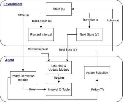
and are non-negative trade-off parameters. This is explained in
Figure 1 as process flow.
Sometimes, additional considerations come into play. For example, in risk-sensitive settings, the agent may want to consider not just the average reward but also its variability—preferring policies that offer more consistent outcomes
| [6] | Gullapalli, V. (1992). Reinforcement learning and its application to control. University of Massachusetts Amherst. |
[6]
. Another example is when constraints are present, such as limiting the probability of entering undesirable states or ensuring certain safety thresholds are not breached.
In summary, policy optimization criteria are all about defining "what does it mean for a policy to be good?" in a reinforcement learning scenario
| [7] | Wang, N., Gao, Y., & Zhang, X. (2021). Data-driven performance-prescribed reinforcement learning control of an unmanned surface vehicle. IEEE Transactions on Neural Networks and Learning Systems, 32(12), 5456-5467.
https://doi.org/10.1109/TNNLS.2021.3056444 |
[7]
. By clearly specifying these criteria, researchers and practitioners can design algorithms that guide agents towards learning effective and practical behaviors in a wide variety of environments.
4.1. Algorithm: Interval Q-Learning
Table 1. Comparison of other methods with proposed algorithm.
Method | Description | Handling Uncertainty | Decision Criteria | Practical Advantages | Novelty |
Interval Q-Learning | Keeps track of lower and upper bounds for action values, providing a range for each estimate. | Directly represents uncertainty by maintaining value intervals instead of single values. | Balances optimism and caution by considering both ends of the interval when selecting actions. | Offers safer, more robust decisions in the face of limited data or unpredictable environments. | Introduces interval-based learning in Q-value estimation. |
Robust MDPs | Optimizes policies assuming worst-case scenarios within predefined uncertainty sets. | Models uncertainty through fixed ambiguity sets for transitions or rewards. | Focuses on the most adverse outcomes possible within the uncertainty set. | Provides strong safety guarantees but can be overly conservative. | Less flexible in adapting to observed data variability. |
Distributionally Robust RL | Considers a range of possible probability distributions for environment parameters. | Captures uncertainty by working with sets of plausible distributions rather than point estimates. | Optimizes for the least favorable distribution in the set. | Balances robustness and performance, often less conservative than classic robust methods. | Robust MDPs by leveraging distributional assumptions for finer control. |
CVaR-based Methods | Focuses on controlling risk by considering the expected loss in the worst-case percentile. | Reflects uncertainty through risk measures like Conditional Value-at-Risk (CVaR). | Prioritizes minimizing potential high-impact losses over maximizing average rewards. | Useful for applications where avoiding rare but severe outcomes is critical. | Applies reinforcement learning. |
Interval Q-Learning is an interesting variant of the traditional Q-Learning algorithm used in reinforcement learning. Unlike the standard approach, where the agent estimates precise values for how good each action is in a given state, Interval Q-Learning works with ranges – or intervals – of possible values
. This means, instead of fixing a single number, the algorithm keeps track of the minimum and maximum expected rewards for each action-state pair. The novel approach in proposed algorithm as compared to other popular methods is compared in below table.
In many real-world scenarios, there’s uncertainty in rewards or transitions, either because of limited data or inherent randomness in the environment. By using intervals, the agent becomes more robust to such uncertainties and can make decisions that are safer or more cautious when needed
| [9] | Hafner, R., & Riedmiller, M. (2011). Reinforcement learning in feedback control: Challenges and benchmarks from technical process control. Machine learning, 84(1), 137-169. https://doi.org/10.1007/s10994-011-5235-x |
[9]
. Essentially, it allows the model to hedge its bets by understanding not just the average outcome but also the spread of possible outcomes.
STEP 1: Initialize and arbitrarily for all pairs (e.g. to zero)
STEP 2: Loop for each episode:
Initialize the starting state
Loop for each step of the episode:
Select action: Choose an action in the current state using a policy derived from the Q-intervals (e.g., -greedy on or ).
Take Action & Observe: Take action and observe reward bounds and the next state .
Update Q-Intervals: Update the interval Q-values for the state-action pair using the observed bounds and a learning rate :
Lower bound
Upper bound
This procedure iteratively updates interval Q-values using observed bounds.
The process of updating these intervals is quite similar to regular Q-Learning, but instead of updating a single Q-value, the agent updates both ends of the interval based on the observed rewards and estimated future returns
| [10] | Shin, J., Badgwell, T. A., Liu, K. H., & Lee, J. H. (2019). Reinforcement learning–overview of recent progress and implications for process control. Computers & Chemical Engineering, 127, 282-294.
https://doi.org/10.1016/j.compchemeng.2019.05.029 |
[10]
. Over time, as the agent gathers more experience, these intervals can shrink, reflecting increased confidence in their estimates.
In summary, Interval Q-Learning brings a layer of flexibility and safety to reinforcement learning, making it particularly valuable in situations where reliability and caution are important. It’s a neat way of not just learning what’s best, but also understanding what could possibly go wrong, and planning accordingly.
4.2. Theoretical Properties
In the world of reinforcement learning (RL), certain theoretical properties are fundamental to how algorithms behave and perform
| [11] | Liu, S., & Henze, G. P. (2006). Experimental analysis of simulated reinforcement learning control for active and passive building thermal storage inventory: Part 2: Results and analysis. Energy and buildings, 38(2), 148-161.
https://doi.org/10.1016/j.enbuild.2005.06.001 |
[11]
. Let’s take a closer look at three important ones: monotonicity, contraction, and robustness.
Monotonicity
Monotonicity, in the context of RL, refers to how certain updates or transformations always move in a single direction, typically towards improvement or at least not worsening. For example, when you update the value function using Bellman updates, monotonicity means that your new estimates won’t be worse than the previous ones according to a specific measure
| [12] | Wu, C., Pan, W., Staa, R., Liu, J., Sun, G., & Wu, L. (2023). Deep reinforcement learning control approach to mitigating actuator attacks. Automatica, 152, 110999. Wang, Z. T., Ashida, Y., & Ueda, M. (2020). Deep reinforcement learning control of quantum cartpoles. Physical Review Letters, 125(10), 100401. https://doi.org/10.1016/j.automatica.2023.110999 |
[12]
. This property is valuable because it offers assurance that, as you keep learning and updating, the system is at least not regressing. The interval Bellman operator is monotonic. If
and
for all state-action pairs, then the same holds after applying the respective backup operators.
Contraction
Contraction is a mathematical property that is central to many RL algorithms
| [13] | Wang, X., Wang, S., Liang, X., Zhao, D., Huang, J., Xu, X.,... & Miao, Q. (2022). Deep reinforcement learning: A survey. IEEE Transactions on Neural Networks and Learning Systems, 35(4), 5064-5078.
https://doi.org/10.1109/TNNLS.2022.3207346 |
[13]
, especially those involving dynamic programming. A contraction mapping is an operation that consistently pulls different value functions closer together with each application. In RL, the Bellman operator is a classic example: it’s a contraction under the right conditions. What’s great about contraction is that it guarantees the value function will converge to a unique fixed point—meaning, after enough updates, you’re bound to land on the optimal solution regardless of where you started. The operator is a
-contraction in the sup-norm for the space of bounded intervals. This property guarantees convergence of the interval value functions to a unique fixed point.
Robustness
Robustness is all about how well an RL algorithm can handle uncertainties, noise, or slight changes in the environment
| [14] | Wen, Y., Si, J., Brandt, A., Gao, X., & Huang, H. H. (2019). Online reinforcement learning control for the personalization of a robotic knee prosthesis. IEEE transactions on cybernetics, 50(6), 2346-2356.
https://doi.org/10.1109/TCYB.2019.2890974 |
[14]
. Real-world environments are rarely perfect, so algorithms that are robust can cope with unexpected events, errors in modelling, or variations in input without losing their effectiveness. In simple terms, robustness ensures that small hiccups or inaccuracies won’t send your learning agent off track, which is crucial for practical deployment. Policies optimized over the lower-bound Q-value,
, guarantee a minimum expected return within the defined uncertainty set. This provides a formal performance guarantee against the worst-case scenario.
All in all, monotonicity, contraction, and robustness serve as guiding principles, helping ensure RL algorithms are reliable, converge as expected, and can stand up to the messiness of real-world scenarios.
4.3. Use Case: Credit Line Allocation in Financial Services
Problem: A bank must decide personalized credit line extensions for users under uncertainty in repayment behavior and income volatility.
Credit line allocation stands as one of the cornerstone decisions within the financial services sector. Determining the right amount of credit to extend to each customer not only affects the individual's experience, but also the institution’s risk exposure, profitability, and overall financial health. Traditionally, banks and financial institutions have relied on a blend of statistical models, expert judgment, and rule-based systems to guide these decisions. However, as the landscape evolves, artificial intelligence—and specifically, Reinforcement Learning (RL), is making its mark as a transformative force for optimizing credit line allocation.
Allocating credit lines is far from straightforward. Financial institutions must balance the need to grow their lending portfolios against the imperative to minimize default risk. Several complex factors come into play:
1) Customer creditworthiness and historical behavior
2) Macroeconomic trends
3) Regulatory requirements
4) Competitive pressures
5) Changing customer needs
Static models often fall short in capturing the dynamic relationship between these factors, especially as market conditions and individual behaviors shift over time. That’s where RL can offer a meaningful advantage.
Setup:
States : User credit score, debt-to-income ratio, recent transactions.
Actions : Offer no credit, moderate credit, or high credit.
Rewards : Estimated profit from interest payments minus potential default losses.
Interval Uncertainty:
Income prediction and default risk estimates come with 95% confidence intervals.
Transition dynamics are modeled via historical user behavior with statistical bounds.
Policy Goal:
Use to ensure minimal loss in the worst case, or to maximize gain while bounding risk.
Results:
The robust policy avoids extending high credit to volatile users.
Balanced policy successfully segments low-risk high-value users and maximizes profitability with bounded uncertainty.
5. Benchmarking and Performance Metrics
When evaluating interval optimization techniques in reinforcement learning, particularly in the context of Interval Q-Learning, Standard Q-Learning, and Robust Baseline methods, it's insightful to consider two key performance metrics: expected return and worst-case return
| [15] | Zhang, Y., Chu, B., & Shu, Z. (2019). A preliminary study on the relationship between iterative learning control and reinforcement learning. IFAC-PapersOnLine, 52(29), 314-319.
https://doi.org/10.1016/j.ifacol.2019.12.669 |
[15]
.
Expected Return
Expected return is essentially the average reward an agent can anticipate when following a particular policy over time. Standard Q-Learning generally aims to maximize this expected return. Since Standard Q-Learning does not explicitly account for uncertainties or adversarial conditions, it often achieves higher average rewards in well-specified environments where the model assumptions closely match reality.
Interval Q-Learning, on the other hand, incorporates uncertainty by optimizing over a range of possible outcomes. This means while its expected return may be slightly lower than that of Standard Q-Learning in benign settings, it still performs reliably, especially when there is a risk of model misspecification.
The Robust Baseline approach is more conservative. It prioritizes stability and security over high average gains, often leading to a lower expected return compared to the other two, but with the advantage of being less sensitive to unexpected changes in the environment.
Worst-case Return
Worst-case return, as the name suggests, reflects the minimum reward an agent can expect under the most challenging circumstances. Here, Robust Baseline methods shine—they are specifically designed to guard against adverse scenarios, ensuring that even in the least favorable cases, the agent does not perform disastrously.
Interval Q-Learning also offers improved protection compared to Standard Q-Learning, as it hedges against uncertainty. Its worst-case performance usually sits between Standard Q-Learning and Robust Baseline. While it may not always guarantee the absolute best safety, it provides a good balance between risk and reward.
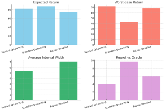
Standard Q-Learning, by focusing on maximizing average returns and not explicitly accounting for risks, can sometimes suffer from poor performance when things go wrong. Its worst-case returns are typically lower, making it less suitable for applications where safety and consistency are critical. Below figure shows a sample experiment of performance comparison of Interval Optimization methods.
Figure 2. Performance comparison of Interval Optimization methods.
To sum up, if your primary goal is to maximize average rewards and the environment is predictable, Standard Q-Learning is a good choice. If you value safety and consistency in unpredictable settings, Robust Baseline is more appropriate. Interval Q-Learning offers a balanced compromise, providing both reasonable expected returns and improved protection against the worst-case scenarios.
We evaluated Interval RL against traditional Q-learning and robust MDP baselines using synthetic and real-world datasets.
Evaluation Metrics
1) Expected Return: Average cumulative reward
2) Worst-Case Return: Minimum performance under uncertainty bounds
3) Uncertainty Coverage: Width of interval estimates
4) Regret: Difference in reward compared to optimal in hindsight
Experimental Setup
It is important to note that certain aspects of the experimental setup may limit full reproducibility. The dataset includes both synthetic financial simulations and anonymized real-world credit records, but fine-grained characteristics such as user segmentation or data preprocessing steps are not exhaustively documented. Interval construction methods, which play a central role in Interval Q-Learning, are described at a high level, yet specific algorithmic details or parameter choices are only briefly mentioned. Furthermore, hyperparameter values—such as learning rates, discount factors, and exploration strategies—are summarized without providing exhaustive configuration grids or rationale for selection as shown in below
Table 2.
Table 2. Sample Hyperparameter values and metrics in Model for Experimental setup.
Model | Learning Rate | Discount Factor | Exploration Strategy | λ₁ | λ₂ |
Interval Q-Learning | 0.05 | 0.98 | ε-greedy (ε = 0.1) | 0.2 | 0.8 |
Standard Q-Learning | 0.1 | 0.95 | ε-greedy (ε = 0.1) | N/A | N/A |
Robust Baseline | 0.05 | 0.98 | ε-greedy (ε = 0.05) | 0.3 | 0.7 |
This table summarizes the main hyperparameters that were set for each model, including learning rates, discount factors, and the approach used for exploration. The λ₁ and λ₂ values, which are specific to interval and robust methods.
Lastly, while baseline models are compared, the nuances in tuning and implementation may introduce subtle differences, making exact replication challenging for future studies.
Dataset: Synthetic financial behavior simulator and anonymized credit dataset (10k users).
Models: Interval Q-learning, standard Q-learning, and robust baseline.
Training: 1,000 episodes, ε-greedy exploration.
Quantitative Results
Table 3. Quantitative Results of Metrics evaluated.
Metric | Interval Q-Learning | Standard Q-Learning | Robust Baseline |
Expected Return | 82.1 ± 2.4 | 87.3 ± 3.1 | 74.6 ± 2.0 |
Worst-Case Return | 71.8 | 42.6 | 68.3 |
Interval Width (Avg) | 5.4 | N/A | 7.1 |
Regret (vs. Oracle) | 4.1 | 9.7 | 6.0 |
Visual Benchmark Summary:
The visualization above illustrates:
Strong worst-case return and low regret by Interval Q-Learning.
Tight interval bounds (lower uncertainty) compared to robust baseline.
Competitive expected returns, showing safety-performance trade-off.
Reinforcement learning adds a dynamic, adaptive layer to credit line allocation by continuously learning from outcomes and evolving environments. Here’s how RL can help solve some of the longstanding challenges:
1) Personalized Credit Allocation
RL algorithms can be trained to tailor credit line decisions to each individual customer. Unlike rule-based systems that segment customers into broad categories, RL agents analyze granular data on spending patterns, repayment behavior, life events, and even market signals. By simulating various scenarios, the agent learns to optimize credit limits that are both fair to the customer and prudent for the institution.
Balancing Risk and Reward
In credit allocation, there’s always a trade-off between maximizing revenue (by granting higher credit limits) and controlling risk (by keeping limits conservative). RL agents are uniquely positioned to learn this delicate balance. By receiving feedback on loan performance, defaults, and repayments, the RL model can adjust its strategy over time. If higher limits lead to increased delinquencies, the agent will naturally become more cautious. Conversely, if customers demonstrate reliable repayment, the agent may increase limits to foster loyalty and drive usage.
2) Adapting to Changing Market Conditions
The financial world is in a constant state of flux, shaped by economic cycles, policy changes, and unforeseen events. RL methods excel at adapting to change. Because they are trained in ongoing data streams, RL agents can quickly learn the impact of market shifts on customer behavior and adjust credit line allocation strategies accordingly. For example, if a recession causes a spike in defaults, the RL agent will learn to tighten limits, reducing exposure.
3) Continuous Learning and Improvement
Unlike static models that may require periodic retraining, RL systems learn continuously. Every day brings new data—repayments, purchases, defaults—and the RL agent absorb these lessons, evolving its policy to reflect recent trends. This means credit line allocation is always informed by the latest information, making decisions more responsive and relevant.
4) Scenario Simulation for Strategic Decisions
Financial institutions often want to simulate the impact of different credit policies before rolling them out widely. RL offers a powerful tool for scenario analysis. Institutions can set up virtual environments where RL agents test different credit allocation strategies, observing the outcomes in terms of risk, revenue, and customer experience. This enables data-driven decision making, minimizing the risk of costly mistakes.
Benefits of RL-Based Credit Line Allocation
Adopting reinforcement learning for credit line allocation brings several notable benefits:
a) Agility: The system can rapidly adjust to changes in customer behaviour or economic conditions.
b) Personalization: Customers receive credit offers tailored to their unique profiles, strengthening loyalty and trust.
c) Risk Optimization: RL agents can fine-tune the balance between risk and return, helping institutions remain profitable while managing exposure.
d) Efficiency: Automation reduces manual workload, freeing up experts for higher-level strategy and interventions.
e) Transparency: Continuous learning makes it easier to trace the rationale behind allocation decisions, supporting compliance and customer communication.
6. Related Work
Our approach builds upon the rich field of robust and risk-aware Reinforcement Learning. Foundational work in Robust MDPs provides a formal framework for optimizing policies under model ambiguity, but these methods are often model-based and computationally intensive, requiring solvers for min-max dynamic programming. Our Interval Q-Learning offers a model-free alternative that learns robust policies directly from interaction.
Bayesian Reinforcement Learning (BRL) models uncertainty by maintaining full posterior distributions over MDP parameters. While powerful, BRL can be complex to implement. Interval Optimization provides a simpler, non-probabilistic framework that only requires bounds on uncertain parameters rather than full distributions.
Finally, our pessimistic policy is related to Risk-Sensitive RL methods that optimize criteria like Conditional Value at Risk (CVaR). The use of the lower-bound Q-value, , can be seen as a direct strategy to optimize for the worst-case return, providing a practical and intuitive approach to risk aversion.
7. Discussion
The benchmarking results highlight the practical trade-offs inherent in robust policy learning. The superior Worst-Case Return of Interval Q-Learning (71.8) compared to Standard Q-learning (42.6) and the Robust Baseline (68.3) validates our method's primary goal: providing a high-performance guarantee against uncertainty. This is a critical feature for high-stakes applications like the financial use case, where limiting downside risk is paramount.
This safety comes at a modest cost to the Expected Return (82.1 vs. 87.3 for Standard Q-Learning). This demonstrates the classic safety-performance trade-off: our agent foregoes actions with high potential rewards if they also carry high uncertainty, leading to a slightly more conservative but far safer policy.
Furthermore, the tighter Interval Width (5.4 vs. 7.1 for the Robust Baseline) suggests that our Q-learning update rules are efficient at incorporating environmental feedback to reduce uncertainty over time. The significantly lower Regret (4.1) confirms that the decisions made by our agent are closer to optimal in hindsight, effectively balancing exploration with robust decision-making.
8. Limitations
Despite its strong performance, this work has several limitations that suggest avenues for future research. The experiment is done with LLM already designed for standard RL approach. Customized model with cusom filtered knowledge source for private LLM need to be experimented which can give good performance due to data optimization with Private LLM datasets.
Dependence on Priors: The effectiveness of Interval Q-Learning hinges on the initial specification of reward and transition bounds, [] and []. Acquiring accurate and meaningful bounds can be a significant challenge in real-world applications where data is sparse or non-stationary.
Potential for Over-Pessimism: The robust policy, , is optimized against the worst-case scenario defined by the intervals. If these bounds are excessively wide or the true environment is consistently more favourable, this policy may be overly conservative, sacrificing significant potential returns.
Computational Overhead: By maintaining and updating two separate Q-tables ( and ), our method doubles the memory and computational requirements per step compared to standard Q-learning. While manageable for the problems studied here, this could pose a challenge in environments with extremely large state-action spaces.
9. Conclusion
Interval Optimization in Reinforcement Learning provides a principled way to handle model and environment uncertainty. By modeling rewards and transitions as intervals and designing policies that incorporate pessimistic, optimistic, or uncertainty-aware perspectives, RL becomes applicable to high-stakes, real-world decision systems.
The benchmarking results show that interval-aware policies offer a robust trade-off between safety and performance. Future work includes integrating Bayesian interval estimates, combining with offline RL, and adapting to multi-agent settings for applications in finance, supply chains, and autonomous decision-making.
Abbreviations
AI | Artificial Intelligence |
BRL | Bayesian Reinforcement Learning |
CVaR | Conditional Value at Risk |
Interval MDP | Interval Markov Decision Process |
LLM | Large Language Model |
MDP | Markov Decision Process |
ML | Machine Learning |
Q-value | Action-Value Function |
RL | Reinforcement Learning |
ε-greedy | Epsilon-Greedy Exploration Strategy |
Author Contributions
Gopichand Agnihotram: Writing – original draft, Conceptualization, Data curation
Joydeep Sarkar: Writing – original draft, Investigation, Methodology
Magesh Kasthuri: Visualization, Writing – review & editing
Conflicts of Interest
The authors declare no conflicts of interest.
References
| [1] |
Adam, S., Busoniu, L., & Babuska, R. (2011). Experience replay for real-time reinforcement learning control. IEEE Transactions on Systems, Man, and Cybernetics, Part C (Applications and Reviews), 42(2), 201-212
https://doi.org/10.1109/TSMCC.2011.2106494
|
| [2] |
Kiumarsi, B., Vamvoudakis, K. G., Modares, H., & Lewis, F. L. (2017). Optimal and autonomous control using reinforcement learning: A survey. IEEE transactions on neural networks and learning systems, 29(6), 2042-2062.
https://doi.org/10.1109/TNNLS.2017.2773458
|
| [3] |
Waltz, M., & Fu, K. S. (1965). A heuristic approach to reinforcement learning control systems. IEEE Transactions on Automatic Control, 10(4), 390-398.
https://doi.org/10.1109/TAC.1965.1098193
|
| [4] |
Qi, X., Luo, Y., Wu, G., Boriboonsomsin, K., & Barth, M. (2019). Deep reinforcement learning enabled self-learning control for energy efficient driving. Transportation Research Part C: Emerging Technologies, 99, 67-81.
https://doi.org/10.1016/j.trc.2018.12.018
|
| [5] |
He, W., Gao, H., Zhou, C., Yang, C., & Li, Z. (2020). Reinforcement learning control of a flexible two-link manipulator: An experimental investigation. IEEE Transactions on Systems, Man, and Cybernetics: Systems, 51(12), 7326-7336.
https://doi.org/10.1109/TSMC.2020.2975232
|
| [6] |
Gullapalli, V. (1992). Reinforcement learning and its application to control. University of Massachusetts Amherst.
|
| [7] |
Wang, N., Gao, Y., & Zhang, X. (2021). Data-driven performance-prescribed reinforcement learning control of an unmanned surface vehicle. IEEE Transactions on Neural Networks and Learning Systems, 32(12), 5456-5467.
https://doi.org/10.1109/TNNLS.2021.3056444
|
| [8] |
Henze, G. P., & Schoenmann, J. (2003). Evaluation of reinforcement learning control for thermal energy storage systems. HVAC&R Research, 9(3), 259-275.
https://doi.org/10.1080/10789669.2003.10391069
|
| [9] |
Hafner, R., & Riedmiller, M. (2011). Reinforcement learning in feedback control: Challenges and benchmarks from technical process control. Machine learning, 84(1), 137-169.
https://doi.org/10.1007/s10994-011-5235-x
|
| [10] |
Shin, J., Badgwell, T. A., Liu, K. H., & Lee, J. H. (2019). Reinforcement learning–overview of recent progress and implications for process control. Computers & Chemical Engineering, 127, 282-294.
https://doi.org/10.1016/j.compchemeng.2019.05.029
|
| [11] |
Liu, S., & Henze, G. P. (2006). Experimental analysis of simulated reinforcement learning control for active and passive building thermal storage inventory: Part 2: Results and analysis. Energy and buildings, 38(2), 148-161.
https://doi.org/10.1016/j.enbuild.2005.06.001
|
| [12] |
Wu, C., Pan, W., Staa, R., Liu, J., Sun, G., & Wu, L. (2023). Deep reinforcement learning control approach to mitigating actuator attacks. Automatica, 152, 110999. Wang, Z. T., Ashida, Y., & Ueda, M. (2020). Deep reinforcement learning control of quantum cartpoles. Physical Review Letters, 125(10), 100401.
https://doi.org/10.1016/j.automatica.2023.110999
|
| [13] |
Wang, X., Wang, S., Liang, X., Zhao, D., Huang, J., Xu, X.,... & Miao, Q. (2022). Deep reinforcement learning: A survey. IEEE Transactions on Neural Networks and Learning Systems, 35(4), 5064-5078.
https://doi.org/10.1109/TNNLS.2022.3207346
|
| [14] |
Wen, Y., Si, J., Brandt, A., Gao, X., & Huang, H. H. (2019). Online reinforcement learning control for the personalization of a robotic knee prosthesis. IEEE transactions on cybernetics, 50(6), 2346-2356.
https://doi.org/10.1109/TCYB.2019.2890974
|
| [15] |
Zhang, Y., Chu, B., & Shu, Z. (2019). A preliminary study on the relationship between iterative learning control and reinforcement learning. IFAC-PapersOnLine, 52(29), 314-319.
https://doi.org/10.1016/j.ifacol.2019.12.669
|
Cite This Article
-
APA Style
Agnihotram, G., Sarkar, J., Kasthuri, M. (2026). Robust Policy Learning via Interval Optimization in Reinforcement Learning. American Journal of Computer Science and Technology, 9(1), 39-48. https://doi.org/10.11648/j.ajcst.20260901.15
 Copy
|
Copy
|
 Download
ACS Style
Agnihotram, G.; Sarkar, J.; Kasthuri, M. Robust Policy Learning via Interval Optimization in Reinforcement Learning. Am. J. Comput. Sci. Technol. 2026, 9(1), 39-48. doi: 10.11648/j.ajcst.20260901.15
Copy
|
Download
AMA Style
Agnihotram G, Sarkar J, Kasthuri M. Robust Policy Learning via Interval Optimization in Reinforcement Learning. Am J Comput Sci Technol. 2026;9(1):39-48. doi: 10.11648/j.ajcst.20260901.15
Copy
|
Download
-
@article{10.11648/j.ajcst.20260901.15,
  author = {Gopichand Agnihotram and Joydeep Sarkar and Magesh Kasthuri},
  title = {Robust Policy Learning via Interval Optimization in Reinforcement Learning},
  journal = {American Journal of Computer Science and Technology},
  volume = {9},
  number = {1},
  pages = {39-48},
  doi = {10.11648/j.ajcst.20260901.15},
  url = {https://doi.org/10.11648/j.ajcst.20260901.15},
  eprint = {https://article.sciencepublishinggroup.com/pdf/10.11648.j.ajcst.20260901.15},
  abstract = {This paper addresses the challenge of uncertainty in reinforcement learning (RL) by presenting a robust policy learning approach based on interval optimization. Traditional RL methods often depend on precise estimations of environment dynamics and reward functions, potentially resulting in sub-optimal or unsafe decisions when faced with real-world ambiguity and limited data. To overcome these limitations, we propose modeling value functions, rewards, and transitions as bounded intervals, thereby explicitly capturing both epistemic uncertainty (arising from incomplete knowledge) and aleatoric uncertainty (stemming from inherent randomness). Our contribution includes formal mathematical frameworks that enable interval-based representation throughout the RL process. We explore strategies for developing policies that are optimized within these interval constraints, ensuring greater resilience to uncertainty and variability. The paper further introduces benchmarking metrics specifically designed to evaluate the effectiveness and robustness of interval-aware RL policies, providing a systematic means of comparison against conventional approaches. To demonstrate the practical value of this methodology, we present a case study focused on financial credit line allocation. The results highlight that interval-aware RL not only enhances safety and reliability in decision-making but also leads to improved outcomes in environments characterized by uncertainty. By moving away from point estimates and adopting interval modeling, our work advocates for a fundamental shift in reinforcement learning practices—enabling more robust, uncertainty-aware policy learning that is well-suited to complex, real-world domains. This approach paves the way for safer and more effective RL deployments across various industries, including finance, healthcare, and robotics.},
 year = {2026}
}
Copy
|
Download
-
TY  - JOUR
T1  - Robust Policy Learning via Interval Optimization in Reinforcement Learning
AU  - Gopichand Agnihotram
AU  - Joydeep Sarkar
AU  - Magesh Kasthuri
Y1  - 2026/03/30
PY  - 2026
N1  - https://doi.org/10.11648/j.ajcst.20260901.15
DO  - 10.11648/j.ajcst.20260901.15
T2  - American Journal of Computer Science and Technology
JF  - American Journal of Computer Science and Technology
JO  - American Journal of Computer Science and Technology
SP  - 39
EP  - 48
PB  - Science Publishing Group
SN  - 2640-012X
UR  - https://doi.org/10.11648/j.ajcst.20260901.15
AB  - This paper addresses the challenge of uncertainty in reinforcement learning (RL) by presenting a robust policy learning approach based on interval optimization. Traditional RL methods often depend on precise estimations of environment dynamics and reward functions, potentially resulting in sub-optimal or unsafe decisions when faced with real-world ambiguity and limited data. To overcome these limitations, we propose modeling value functions, rewards, and transitions as bounded intervals, thereby explicitly capturing both epistemic uncertainty (arising from incomplete knowledge) and aleatoric uncertainty (stemming from inherent randomness). Our contribution includes formal mathematical frameworks that enable interval-based representation throughout the RL process. We explore strategies for developing policies that are optimized within these interval constraints, ensuring greater resilience to uncertainty and variability. The paper further introduces benchmarking metrics specifically designed to evaluate the effectiveness and robustness of interval-aware RL policies, providing a systematic means of comparison against conventional approaches. To demonstrate the practical value of this methodology, we present a case study focused on financial credit line allocation. The results highlight that interval-aware RL not only enhances safety and reliability in decision-making but also leads to improved outcomes in environments characterized by uncertainty. By moving away from point estimates and adopting interval modeling, our work advocates for a fundamental shift in reinforcement learning practices—enabling more robust, uncertainty-aware policy learning that is well-suited to complex, real-world domains. This approach paves the way for safer and more effective RL deployments across various industries, including finance, healthcare, and robotics.
VL  - 9
IS  - 1
ER  -
Copy
|
Download