Mathematical Modeling of the Amplitude Dynamics of Saturated Sludge in a Landslide Wave Surge

David Pkiach Karugutiang; Cleophas Kweyu; Christopher Kaneba

doi:doi:10.11648/j.ajam.20261402.16

Research Article |

| Peer-Reviewed

Mathematical Modeling of the Amplitude Dynamics of Saturated Sludge in a Landslide Wave Surge

David Pkiach Karugutiang^*

, Cleophas Kweyu

, Christopher Kaneba

Published in American Journal of Applied Mathematics (Volume 14, Issue 2)

Received: 17 January 2026 Accepted: 5 February 2026 Published: 13 April 2026

Views: Downloads:

Download PDF

Share This Article

Twitter
Linked In
Facebook

Abstract

Mathematical model is formulated using Partial differential equations, and analyzed to describe the dynamics of wave propagation with application to landslide. Its occurrence leads to loss of lives of people and their properties. This study aims at understanding the dynamics of landslide wave propagation, in order to make adequate projection in an attempt to mitigate the risks involved in the occurrence. The objective of this study is; to develop a mathematical model to describe the dynamics of a landslide wave propagation. Numerical solutions were carried out using Runge-Kutta algorithm’s inbuilt in MATLAB, to simulate the current and future dynamics of the model. The mathematical model was used to simulate and analyze landslide wave propagation phenomena in affected areas. The results of this study showed that the maximum amplitude of 0.49m is achieved at an inclination of 50° and gradually drops down to 0.45m at a slope of 19.2°. This defines the region where inhabitants should be relocated to avoid loss of lives and destruction of property during the occurrence of landslide. The high amplitude occurs in the wave propagation region, necessitating the implementation of control strategies along the same region.

Published in	American Journal of Applied Mathematics (Volume 14, Issue 2)
DOI	10.11648/j.ajam.20261402.16
Page(s)	79-87
Creative Commons	This is an Open Access article, distributed under the terms of the Creative Commons Attribution 4.0 International License (http://creativecommons.org/licenses/by/4.0/), which permits unrestricted use, distribution and reproduction in any medium or format, provided the original work is properly cited.
Copyright	Copyright © The Author(s), 2026. Published by Science Publishing Group

Keywords

High Landslide Mobility, Amplitude, Momentum, Conservation, Laboratory Flume

1. Introduction

Landslide waves are among the most devastating natural disasters, causing destruction of infrastructure, displacement of communities, and loss of human life. They commonly occur in areas with steep slopes, especially where human activities such as deforestation have destabilized the terrain. In Kenya, West Pokot County is a prime example of a region prone to recurrent landslides due to its escarpment landscapes and high rainfall. The movement of saturated soil, rock, and debris under gravitational pull forms a landslide. This mass can generate a surge wave when it rapidly displaces water in its path. These waves, characterized by extreme mobility and amplitude, have the potential to overtop natural or artificial dams, exacerbate flooding, and spread debris over vast distances. Understanding the dynamics of such waves is critical for predicting their impact and designing effective mitigation strategies. However, modeling such complex, nonlinear fluid-solid interactions pose challenges due to factors such as turbulence, terrain irregularities, and heterogeneous soil structures. This study aims to develop and validate a robust mathematical and computational model to simulate landslide-induced surge wave propagation using experimental fluid dynamics and numerical methods.

2. Literature Review

Landslides and their associated surge waves have been the subject of extensive global research due to their destructive nature and complex dynamics. Prior studies have investigated the mechanisms of landslide initiation, wave generation, and propagation using a variety of theoretical, numerical, and experimental approaches. However, significant limitations remain in accurately in modeling and predicting landslide-induced surge wave behavior in real-world conditions, especially in developing countries such as Kenya. The researcher laid the foundation for understanding landslide mechanics, identifying gravitational movement of soil and rock as the principal cause

[19]

. The study expanded on this, classifying landslide types and emphasizing their dependence on geo- logical and hydrological factors

[19]

. Later studies, such as those by

[3]

, confirmed that landslides can occur across various environments, including off-shore and onshore regions.

Recent investigations

[23]

highlighted that rainfall-induced changes in pore water pressure are key triggers of shallow landslides. While these findings are essential, they largely focus on landslide initiation rather than the propagation phase of landslide surge waves. Moreover, these studies seldom account for landslide mobility or the rheological behavior of highly viscous mudflows during long distance travel.

Zhou, S. et al. discussed the role of rainfall intensity and soil saturation in slope failure

[23]

. Their work, although insightful, primarily relies on empirical correlations and does not delve into detailed dynamic modeling of surge waves post-landslide. Similarly,

[17]

and

[7]

recognized the significance of soil-water interaction and capillary forces in slope instability, but these studies do not adequately address how such conditions influence wave energy transmission downstream. In analyzing landslide processes, two methods are preferred. The first approach employs statistical inferences to establish the relationship between rainfall characteristics and landslide event probability while the second method employs physical mechanisms of the rainfall infiltration or soil water content variation to trigger landslide events

[15]

Tsunami-like waves caused by landslides have also attracted interest.

It was concluded that the 1998 Papua New Guinea tsunami was more likely triggered by an underwater landslide than the earthquake itself

[15]

. These conclusions underscore the need to focus on surge wave modeling rather than seismic parameters alone. Nevertheless, these studies lack an integrated approach that combines both experimental validation and dynamic simulation for inland landslides. Experimental investigations by

[8, 23]

, and

[22]

demonstrated how physical models could replicate wave behaviors under controlled conditions. The researcher advanced this by considering the shape and volume of landslide bodies

[5]

. The researcher presented the results of his experiment in a 2-D Blume, in which it showed that the landslide surge wave might be more serious than that directly caused by the earthquake, and could be hazardous to human life

[21]

. In another 2 D experiment,

[20]

presented the landslide body that consisted of a triangular front and a rectangular tail, which made the body volume adjustable. While useful, these experiments were primarily limited to 2D models and assumed idealized boundary conditions that may not reflect natural terrain variability. Numerical approaches, including the Boussinesq and Navier–Stokes models, have been developed to simulate landslide-induced wave dynamics

[11]

and

[5]

The researcher conducted a numerical study using his NASA-VOF2D model based on the Navier-Stokes (NS) equations

[7]

. In this model, the motion of the landslide was experimented, a comparison between numerical and experimental results was presented. The numerical model for the landslide-induced wave needs proper simulation of dynamic fluid-structure and water wave propagation

[1]

. In the above mesh-based models, the Lagrangian landslide body motion is described in a Euler grid, and the movement of the body-fitted grid near the structure and the communication between the moving body and the Eulerian meshes, increased the algorithm complexity. This method has been widely used in many hydrodynamics problems

[13]

but so far there has been little application of SPH to landslide surge wave simulation.

In particular, the Smooth Particle Hydrodynamics (SPH) and Incompressible SPH (ISPH) methods have gained attention for their ability to model complex free-surface flows

[12, 14]

. However, most of these studies treat landslide motion as a known input either as a predefined function, a constant value, or experimental data

[4, 6, 16]

. This assumption significantly limits their predictive capacity in real-time hazard assessment, where landslide motion is inherently uncertain and spatially variable. The researcher attempted to overcome this by introducing coupled fluid- structure interaction in ISPH models

[10]

. However, their models do not fully simulate boundary contact, which is critical in terrain-influenced landslide propagation. Additionally, while

[2]

pointed out that surge wave propagation remains underrepresented in SPH literature, few studies have tackled this omission systematically, particularly for high-mobility mudflows in steep, vegetated terrains common in tropical highlands.

Regionally, studies in Kenya have focused more on landslide risk mapping and environmental triggers

[8, 11, 18]

with minimal integration of mathematical or computational modeling. These studies highlight critical anthropogenic triggers like deforestation, slope modification, and poor drainage, but they do not provide dynamic predictions of landslide wave impacts. This lack of predictive modeling limits the ability of policymakers and engineers to implement timely mitigation strategies. Heavy rainfall was experienced in the border of Elgeyo Marakwet and West Pokot Counties that caused landslide, claimed the lives many people and destroyed of properties.

This paper investigates the dynamics of landslide- induced wave propagation, underscoring mathematical models approaches, particularly the Incompressible Smooth Particle Hydrodynamics (ISPH) method using numerical model. By comparing experimental results with numerical simulated results of high and low mudflow mobility that produce amplitude waves of different magnitudes. This research combines experimental validations and numerical simulations to predict landslide processes and inform effective mitigation strategies and applying it to a Kenyan terrain setting, the research provides a robust framework for early warning, infrastructure planning, and environmental risk management. Moreover, the influence of fluid-solid interaction, turbulence, and variable terrain slopes on surge wave amplitude and runout distance remains insufficiently explored, especially in the African context. Therefore, this study fills a critical gap by integrating experimental fluid dynamics with ISPH based numerical modeling to simulate source, middle and far-field landslide wave propagation.

3. Dynamic Model for Landslide Propagation

The SPH 2-D depth-integrated numerical model was adopted for predicting the runout distance of mud-flow, flow velocity, composition of the deposition and final volume of mudflow

[12]

. The model solved three-dimension Navier Stokes equation using Fourier transform methods. Numerical solution was carried out using Runge-Kutta algorithm’s inbuilt in MATLAB, to simulate the current and future dynamic models, it predicted the runout distance of mud-flow, velocity, composition of the deposition and final volume of mudflow.

3.1. Governing Equations for Landslide Propagation

The empirical model for precipitation representing a single rainfall event over a period of time was derived from an odd Fourier Series expression

[9]

Rη (t) = \frac{k}{η} \sum_{η = 1}^{\infty} \frac{sin (2 η -1) t}{(2 η - 1)}

(1)

where k and

η

are curve fitting parameters, determined from experimental validations. The general equation of conservation of mass satisfies the Laplacian equation

[10]

η ρ_{m} \nabla . u = 0

(2)

where

u

is the particle velocity vector,

\nabla

is the three-dimensional divergence operator,

ρ_{m}

is the density of the mixed fluid,

η

is the height or the amplitude wave surface, while

t

is time in seconds.

The differential expression derived from the conservation of Momentum;

\frac{\partial u}{\partial t} = - \frac{1}{ρ_{m}} \nabla p + g + μ \nabla^{2} u + \frac{1}{ρ_{m}} \nabla . τ

(3)

where

u

is the particle velocity vector

t

is the time,

ρ_{m}

is the density of fluid,

p

is the particle pressure,

g

is the gravitational acceleration vector,

μ

is the laminar kinematic viscosity and

τ

is the sub particle scale (SPS) turbulence stress

[14]

3.2. Energy

The energies of waves generated by the landslide is the sum of both kinetic energy and potential energy of vibration. The potential energy of high mobility mudflow wave and kinetic energy of also high mobility mudflow wave produced by the landslide body entering water are described as follows:

E_{p} = \frac{1}{2} {bρ}_{ω} gc \int_{0}^{l} η^{2} dt

(4)

E_{k} = \frac{1}{2} m_{s} v_{s}^{2}

(5)

E_{p}

denote the potential energy, where b is the width of the landslide body, and c is the wave velocity

E_{k}

refers to kinetic energy of water percolating through the rocks.

v_{s}

is the speed of the fluid entering soil,

η

is wave height,

ρ_{ω}

is the density of water

m_{s}

mass of the sliding body and

g

is the gravitational density.

3.3. Eddy Viscosity

Eddy viscosity or turbulent viscosity did not physically exist but its concept is introduced to simplify the analysis of turbulent flow. The eddy viscosity assumption is used to model sub-particle scale turbulence stress

τ

[13]

as,

τ_{ij} = ρ_{m} (2 v_{t} s_{ij} - \frac{2}{3} k δ_{ij})

(6)

Where

v_{t}

is the turbulence eddy viscosity,

s_{ij}

is the strain rate tensor,

k

is the turbulence kinetic energy and

\partial_{ij}

is the Kronecker delta functions. The eddy viscosity

v_{t}

is calculated using a modified Smagorinsky model

[9]

v_{τ} = {(C_{s} d_{0})}^{2} | S |

(7)

where

C_{s}

is the Smagorinsky constant,

C = 0.1

and

d_{o}

is the particle spacing representing the characteristic length scale of the small eddies.

|s| = \sqrt{(2 s_{ij} s_{ij})}

isthelocalstrainrate.(8)

This method is used solve equation (2) and (3) as outlined in

[14]

. This computation is composed of two steps. The first step is an explicit integration of velocity in time without considering the pressure and gravity.

u_{*} = u_{t} + (v_{o} \nabla^{2} u + \frac{1}{ρ} \nabla τ) ∆ t

(9)

r_{*} = r_{t} + u_{*} ∆ t,

(10)

Where

u_{t}

and

r_{t}

are particle velocity and position at time

t

, while

u_{*}

and

r_{*}

are the intermediate particles velocity and

∆ t

is the time increment.

Assuming that

{∆ u}_{* *}

is the changed particle velocity contributed by the remaining pressure and gravity.

u_{t + 1} = u_{*} + u_{* *} = u_{*} + (g - \frac{1}{ρ} \nabla p_{t + 1}) ∆ t

(11)

Through the combination with the mass conservation equation (2), the pressure Poisson Equation (PPE) is obtained as

[10]

\nabla . (g - \frac{1}{ρ} \nabla p_{t + 1}) = - \frac{\nabla u_{*}}{∆ t}

(12)

After obtaining the pressure field, the particle velocity was updated by equation (11) and the position of the particle are centered in time as

r_{t + 1} = r_{t} + (\frac{u_{t} + u_{t + 1}}{2}) ∆ t

(13)

3.4. Incompatible Smooth Particle Hydrodynamics (ISPH) Formula

The viscous and the turbulent terms in equation (3) are given by

[13]

;

(

{v_{o} \nabla^{2} u)}_{t} = \sum_{j} (\frac{4 m_{j} (u_{i} + u_{j}) r_{ij} . \nabla_{i} w_{ij}}{{(ρ_{i} + ρ_{j})}^{2} ({r_{ij}}^{2} + η^{2})}) u_{ij}

(14)

(\frac{1}{ρ} \nabla . τ) = \sum_{j} (m_{j} (\frac{τ_{i}}{{ρ_{i}}^{2}} + \frac{τ_{j}}{{ρ_{j}}^{2}}) . \nabla_{i} w_{ij}

(15)

Where

i

and

j

are reference particles,

m

is the mass of the particle,

w

is the kernel function and

μ

is the dynamic viscosity. This is equal to;

{ρv}_{o} . r_{ij} = r_{i} - r_{j, u_{ij}} = u_{i} - u_{j}

where

η

is 0.1h. h is the smoothing length and

\nabla_{i} w_{ij}

is the kernel gradient. The pressure term

[13]

, is expressed as

{\frac{1}{ρ} \nabla p}_{i} = \sum_{j} m_{j} (\frac{p_{i}}{{ρ_{i}}^{2}} + \frac{p_{j}}{{ρ^{2}}_{j}}) \nabla_{i} w_{ij}

(16)

The velocity divergence I the right-hand side of the equation (12)

[14]

is discretized as

(\nabla {u_{*})}_{i} = \sum_{j} \frac{m_{j}}{ρ_{j}} (u_{* i} - u_{* j}) \nabla_{i} w_{ij}

(17)

And the left-hand side of equation (3) is expressed as

\nabla . (\frac{1}{ρ} \nabla p) = \sum_{j} \frac{{8 m}_{j}}{{{(ρ}_{i} + ρ_{j})}^{2}} - \frac{p_{ij} r_{ij}}{(| {r_{ij} |}^{2} + η^{2})}) \nabla_{i} w_{ij}

(18)

Where

p_{ij} = p_{i} - p_{j}

The choice of different kernel function can greatly affect smooth particle hydrodynamics performance, just like the different Finite Difference Method in this proposed two-Dimensional Incompatible Smooth Particle Hydrodynamics (2DISPH) method, the B-spline kernel function was used.

w (q, h) = [\begin{matrix} \frac{15}{7 π h^{2}} (\frac{2}{3} - q^{2} + \frac{1}{3} q^{3}) 0 < q < 1.0 \\ \frac{15}{7 π h^{2}} ({\frac{1}{6} (2 - q^{3})}^{3} 1.0 < q < 2.0 \\ 0 q \geq 2.0 \end{matrix}]

(19)

Where

q = \frac{| r_{i -} r_{j} |}{h}

3.5. Landslide Model Establishment

Using

[10]

, fluid pressure in the sliding body is integrated using the pressure integration procedure to get fluid force F_fon the grid body. The sliding fluid sliding towards the landslide is perpendicular to the F_s. This meant that supported force made no contribution to the sliding velocity.

F_{res} = G^{incline} - {F_{s}}^{incline}

. Where

G^{incline}

and

{F_{f}}^{incline}

are the components of G and

F_{s}

respectively.

F_{res}

is the resultant force on the direction of the movement. In fluid, solid coupling using smooth particle hydrodynamic method, moving boundary is not allowed to contact the fixed boundary

[1]

. In landslide sliding, fluid slide in an inclination, it made the moving boundary shorter to the fixed boundary.

3.6. The Free Treatment of Surface

Free treatment of surface, Dirichlet boundary condition

ρ

=constant is added where the constant

p

denotes the atmospheric pressure. Using

[9]

, the free treatment of surface was as

({ρ (number)}_{i} = \sum_{j} w (|r_{i} - r_{j}|) h) dv

(20)

({ρ (smp)}_{i} = \sum_{j} \frac{m_{j}}{ρ_{j}} \frac{x_{ij} + z_{ij}}{d_{o}} w (|r_{i} - r_{j}|) h)

(21)

Where

ρ

number is the particle number density that was close to 1.0 in the inner fluid region, dv is the volume of the particle and

dv = \frac{m_{j}}{ρ_{j}} j

, where

ρ

number

< 0.9

, the particle is the surface particle.

x_{ij} = x_{i}

x_{j}

z_{ij} = z_{i -} z_{j}

(22)

ρ sym

is the quantification of the particle distribution a symmetry, and the critical value was chosen as 0.1 for the inner fluid particle in the present model.

4. Model Application and Validation

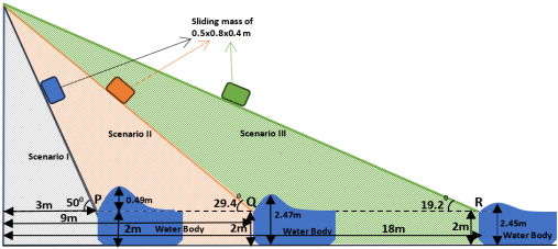
In this section, mudflow experiments were conducted in the laboratory using flume as shown in Figure 1. To validate the performance of the numerical simulation, the physical experiment by

[7]

was used as the reference standard for comparison. The density of the sliding mass was 2282

{kg / m}^{3}

. The mudflow model input data is shown in Table 1. Results of the three points P (

x = 3 m

), Q (

x = 6 m

) and R (

x = 9 m

) for free surface variation were extracted and compared with the results of physical experiment model for validation.

Download: Download full-size image

Figure 1. Experimental diagram for the validation in (m).

4.1. Initial and Boundary Conditions

The table below shows different parameter measurements used in a landslide experiment.

Table 1. Landslide model input data.

Related parameters	Specific numerical
Density of slide block (kg/m³⁾	2282
Coefficient of friction	0
Grid size (m)	0.05
Sliding mass dimensions (m)	0.5 x 0.8 x 0.4
Depth of the water (m)	2.0

4.2. Control Equation of Mudflow Propagation Process

Conservation mass equation as seen in equation (2)

η \nabla ρ_{ω} . u = 0

where u is the particle velocity.

\nabla

is the divergence operator.

ρ_{ω}

is the density of water. This gave rise to differential expression derived from the conservation of Momentum as drafted in equation (3)

\frac{\partial u}{\partial t} = \frac{- 1}{ρ_{m}} \nabla p + g + μ \nabla^{2} u + \frac{1}{ρ_{m}} \nabla . τ

Computational model had boundary limits set since the solid walls had not slip limit, the fluid velocity.

gradient and its flow variables were fixed to be zero at the fluid-solid interface. The upper art of the laboratory flume was fixed as a free surface boundary. It meant that the liquid pressure was equal to gas pressure, the normal velocity on the free surface was set to be zero. The other four boundaries corresponding and their flow flux and shear stress was equal to zero. Water surface was not impacted by landslide body and remained stationary. Initially the speed of the landslide body was zero.

Three experiments were conducted for points P (

x = 3 m

), Q (

x = 9 m

) and R (

x = 18 m

) and their numerical results were compared for future use in landslide prediction.

4.3. Experimental Results for Point P (x = 3m)

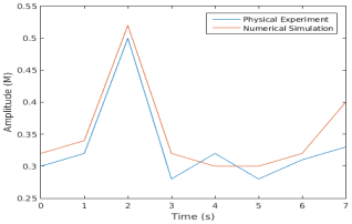
Table 2. Landslide near field amplitude results at point p (x = 3 m).

Time (s)	0	1	2	3	4	5	6
Experimented amplitude [m]	0.30	0.31	0.49	0.28	0.32	0.29	0.30
Numerical amplitude [m]	0.31	0.31	0.50	0.29	0.33	0.30	0.31

Download: Download full-size image

Figure 2. Comparison of amplitude wave at point P (

x = 3 m

4.3.1. Observation and Results at Point P (x=3m)

After drawing the graph using the extracted results for point P (

x = 3 m

) Table 2, it was observed that the experiment reached maximum height of 0.49 m and the numerical simulation showed that the maximum crest was 0.50 m on free guided lubricated laboratory flume. The amplitude of the experiment reached the crest after 2 seconds. It produced relative error of 2% compared to the experimental results. The trough reached a minimum of 0.28 m. It appeared after 3 seconds. The calculated physical experiment results were consistent with numerical results. High mobility mudflow produced high amplitude waves (crest) and lower troughs, with minimum amplitudes change as waves propagated from the source.

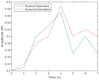
Table 3. Mudflow midfield amplitude results at point q (

x = 9 m

Time (s)	0	1		2	3	4	5	6	7
Experimented Amplitude [m]	0.3	0.31		0.31	0.35	0.47	0.26	0.35	0.33
Numerical amplitude [m]	0.3	0.31		0.31	0.36	0.48	0.27	0.3.6	0.34

Download: Download full-size image

Figure 3. Comparison of amplitudes fluid at point Q (x=9m).

4.3.2. Observation and Results at Point Q (x=9m)

Figure 3, showed experimented results for point Q which had maximum amplitude of 0.47m that occurred 4th second, while numerical simulation produced peak height of 0.48m at 4th second. Both experimented and numerical results showed a decay in maximum amplitudes. It produced relative error of 2% compared to the experimental result. Both produced similar peak height, which was lower than the amplitude for point P. The second experimented amplitude for point Q was 0.35m that occurred at 6^th second, while numerical simulation produced amplitude of 0.37m at 6^th second. Both showed decay in other subsequent amplitudes due to decrease in gradient and reduced interparticle collision. There was a decrease in experimented amplitude for point Q (0.47m) compared to the amplitude at point P (0.49m). The flume bottom and side walls were lubricated hence there was no friction. Physical experiment produced trough of 0.26m at the 5^th second and for numerical simulation it produced a trough 0.27m at 5^th second. Experimented results and numerical results showed similarity in amplitudes. The plastic container stopped the sliding block from hitting the bottom of the flume. Energy dissipation and collision was neglected in numerical simulation between block and baffle.

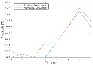
Table 4. landslideresults for far field at point c

(X = 18 m)

Time(s)	0	1	2	3	4	5	6	7
Experimented Amplitude [m]	0.30	0.31	0.32	0.34	0.34	0.37	0.45	0.25
Numerical amplitude [m]	0.3	0.33	0.33	0.35	0.44	0.37	0.47	0.27

Download: Download full-size image

Figure 4. Comparison of amplitudes fluid for far field at point R (x=18).

4.3.3. Observation and Results at Point R (x = 18m)

The velocity of the sliding block for point R moved relatively slowly compared to the velocity at point Q due to decreased gradient and weakened interparticle collision. It reached its maximum amplitude of 0.45 m experimentally and 0.47 numerically at point R that occurred at 6 second. It had amplitude difference of 0.2m with relative error of 4.255% compared to experimental results. There was low landslide mobility with decayed amplitudes. It also showed lower crest for both experimented and numerical results at point R that appeared after 7 second. The comparison analysis showed that the peaks for points Q for both numerical and experimental analysis was the same, showing that the calculation results were consistent with the physical experiment.

4.4. Discussion

Figure 2 shows landslide conditions at point P, analogous to a triggering zone with prolonged rainfall reducing soil friction and strength, leading to collapse. The experimental amplitude (0.49 m) closely matched the numerical simulation (0.50 m), with a 2% error. These reduced amplitude waves propagation for points P, Q and R were caused by decreased particle collision and energy dissipation down the slope. Energy dispersion was transferred partially from the main peak progressively towards the trailing wave

[10]

. High-mobility mudflow slides rapidly down the steep slope and produced high-amplitude waves.

At point Q (Figure 3), experimental and numerical amplitudes were 0.47 m and 0.48 respectively, it had low amplitude compared to point P. High mudflow mobility on steep slopes generated high-amplitude waves over long runout distances. Increased porosity reduced near-field amplitude due to deceleration

[12]

. Velocity peak on steep gradients, enhancing erosion. The densities of the three points P, Q and R showed progressive reduction in amplitude waves because the density of point P (near field) generate high kinetic energy compared to the other far field.

Figure 4 shows low landslide mobility at point R, with a maximum amplitude of 0.45m which had decayed further due to weakened interparticle collisions and decreased velocity resulting to high deposition of sand and mudflow features. The comparison analysis shows that the occurrence times for both amplitude waves in numerical simulation and experimentation were the same. This showing that the calculation results were the same with physical experimentation. Sand deposits are very important economically since its used for construction purposes and generated income to the people in the landslide deposit region. Erosion control measures, such as afforestation and retaining walls, stabilize slopes and restrict settlement in high-risk areas.

5. Summary and Conclusions

The results from the experimental and numerical simulations, as presented in Figures 2 to 4, demonstrate the efficacy of the Incompressible Smoothed Particle Hydrodynamics (ISPH) model in solving the dynamics of landslide-induced surge waves. It showed similarity to

[8]

test results. At point P (

x = 3 m

), there is close agreement between experimental (0.49m) and numerical (0.50 m) maximum amplitudes, with a 2% relative error, validates the model’s accuracy in triggering zone, where high-mobility mudflows generate significant amplitude waves due to rapid energy transfer from the sliding block

[9]

. The observed amplitude decay at point Q (

x = 9 m

), experimental results of 0.47 m and numerical results of 0.48 while point R (

x = 18 m

), experimental results of 0.45 m and numerical results of 0.467m reflects the dissipation of wave energy as the mudflow progresses to the runout and deposition zones, consistent with reduced landslide mobility and increased frictional effects

[23]

. These findings align with the literature, where wave amplitude attenuation is attributed to factors such as bottom friction and material deposition

[1]

. The ISPH models’ ability to simulate complex fluid-solid interactions, as detailed in the methodology section, addresses limitations in prior models that often assume predetermined landslide motion

[11]

and

[4]

. By incorporating dynamic coupling between the landslide body and fluid, the model provides a more realistic representation of surge wave propagation, particularly in scenarios involving contact with fixed boundaries

[15]

. The use of Fourier transforms methods and Runge-Kutta algorithms in MATLAB, as described in the abstract, enabled precise numerical solutions, capturing the viscous and turbulent flow characteristics of the landslide fluid mixture (Table 1). The models stability and sensitivity to perturbations, tested as part of the methodology, further enhance its reliability for predictive applications.

This study developed and validated a mathematical model using partial differential equations and the ISPH method to simulate landslide-induced surge wave propagation. The model accurately predicted amplitude waves like 0.49m at point P, 0.47m at point Q, 0.45m at point R with minimal error compared to experimental results, demonstrating its reliability in capturing the dynamics of high-mobility mudflows. These reduced amplitude waves propagation for P, Q and R were caused by decay in in energy down the slope. Energy dispersion was transferred partially from the main peak progressively towards the trailing wave

[10]

By addressing gaps in prior models, such as predetermined landslide motion, the ISPH approach provides a more realistic simulation of fluid-solid interactions, as evidenced by the results in Figures 2 to 4. The findings enhance the ability to predict landslide occurrences and their impacts, supporting early warning systems and mitigation strategies like afforestation and structural reinforcements. This work improves existing models and offers a valuable tool for researchers and policymakers to protect lives, properties, and economic livelihoods in landslide-prone regions.

The contribution of research work is based on conceptualization, dynamic model and validation, landslide behavior and the conclusion. (2) The contribution of methodology in the calculation of and simulation landslide amplitudes (3) The contribution of results based on computation experimental study for generation of high amplitude and low amplitude waves.

Abbreviations

D.K	David Karugutiang
C.K	Cleophas Kweyu
K.C	Kaneba Christopher

Author Contributions

David Pkiach Karugutiang: Conceptualization, Data curation, Formal Analysis, Investigation, Project administration, Resources, Software, Visualization, Writing – original draft

Cleophas Kweyu: Methodology, Project administration (planning), Validation, Writing – review & editing

Christopher Kaneba: Project coordination, Writing – review & editing

Data Availability Statement

The original contributions presented in this study are included in the article material, further inquiries can be directed to the corresponding author.

Conflicts of Interest

The author declares no conflicts of interest.

References

[1]	Ataie-Ashtiani, B., & Shobeyri, G. Numerical simulation of landslide impulsive waves by incompressible smoothed particle hydrodynamics. International Journal for Numerical Methods in Fluids (2008) 56(2): 209-232.
[2]	De Girolamo, P., Wu, T.-R., Liu, P. L.-F., Panizzo, A., Bellotti, G., & Di Risio, M. Numerical simulation of three-dimensional tsunamis water waves generated by landslides: Comparison between physical model results, VOF and SPH. In Coastal Engineering (2007) 2006: (In 5 Volumes) (pp. 1516-1528). World Scientific.
[3]	Deschamps, R. J. A study of slope stability analysis. Purdue University (1993).
[4]	Enet, F., Grilli, S. T., & Watts, P. Laboratory experiments for tsunamis generated by underwater landslides: comparison with numerical modeling. ISOPE International Ocean and Polar Engineering Conference (2003), ISOPE--I.
[5]	Grilli, S. T., & Watts, P. Tsunami generation by submarine mass failure. I: Modeling, experimental validation, and sensitivity analyses. Journal of Waterway, Port, Coastal, and Ocean Engineering 1 (2005) 31(6), 283-297.
[6]	Guzzetti, F., Ardizzone, F., Cardinali, M., Rossi, M., & Valigi, D. Landslide volumes and landslide mobilization rates in Umbria, central Italy. Earth and Planetary Science Letters (2009) 279(3-4), 222-229.
[7]	Heinrich, P. Nonlinear water waves generated by submarine and aerial landslides. Journal of Waterway, Port, Coastal, and Ocean Engineering (1992) 118(3), 249-266.
[8]	Li, T., Troch, P., & De Rouck, J, (2004). Wave overtopping over a sea dike. Journal of Computational Physics, 198(2), 686-726.
[9]	Liu, X., Lin, P., & Shao, S. An ISPH simulation of coupled structure interaction with free surface flows. Journal of Fluids and Structures, (2014) 48, 46-61.
[10]	Liu, X., Xu, H., Shao, S., & Lin, P. An improved incompressible SPH model for simulation of wave--structure interaction. Computers \& Fluids (2013). 71, 113-123.
[11]	Nduru G. M. Evaluation of Spatial Variation in Landslide Potential within South Mathioya Drainage Basin, Kenya. M. Phil thesis, Moi University, Eldoret, Kenya (1995).
[12]	Pastor, M., Haddad, B., Sorbino, G., Cuomo, S., & Drempetic, V. A depth-integrated, coupled SPH model for flow-like landslides and related phenomena. International Journal for Numerical and Analytical Methods in Geomechanics (2009) 33(2), 143-172.
[13]	Shao, S. Incompressible SPH simulation of water entry of a free-falling object. International Journal for Numerical Methods in Fluids (2009) 59(1), 91-115.
[14]	Shao, S., & Gotoh, H. Simulating coupled motion of progressive wave and floating curtain wall by SPH-LES model. Coastal Engineering Journal (2004) 46(02), 171-202.
[15]	Okal, E. A. T. waves from the 1998 Papua New Guinea earthquake and its aftershocks: Timing the tsunamigenic slump. Landslide Tsunamis: Recent Findings and Research Directions (2003) 1843-1863.
[16]	Sue, L. P., Nokes, R. I., & Davidson, M. J. Tsunami generation by submarine landslides: comparison of physical and numerical models. Environmental Fluid Mechanics (2011) 11, 133-165.
[17]	Terzaghi (1962), Weissel, J. K., & Seidl, M. A. Influence of rock strength properties on escarpment retreat across passive continental margins. Geology (1997) 25(7), 631-634.
[18]	Ucakuwun, E. K., Munyao, T. M., Simiyu, G. M., Esipila, T. A.,&Chepkosgei, E. Landslide occurrences in Khuvasali, Kakamega North District, Kenya. Unpublished paper presented at the 4thMoi University Annual Conference, held at Moi University, August 2008.
[19]	Varnes, 1996. Hungr, O., Leroueil, S., & Picarelli, L. (2014). The Varnes classification of landslide types, an update. Landslides, 11, 167-194. Varnes, 1996. Hungr, O., Leroueil, S., & Picarelli, L. (2014). The Varnes classification of landslide types, an update. Landslides, 11, 167-194.
[20]	Walder, J. S., Watts, P., Sorensen, O. E., & Janssen, K. Tsunamis generated by subaerial mass flows. Journal of Geophysical Research: Solid Earth (2003) 108(B5).
[21]	Wiegel, R. L. Laboratory studies of gravity waves generated by the movement of a submerged body. American Geophysical Union-Transaction (1955) 36(5), 759-774. https://doi.org/10.1029/TR036i005p00759
[22]	Xu, X. Z., Guo, W. Z., Liu, Y. K., Ma, J. Z., Wang, W. L., Zhang, H. W., & Gao, H. Landslides on the Loess Plateau of China: a latest statistic together with a close look. Natural Hazards (2017) 86(3), 1393-1403.
[23]	Zhou, S., Zhou, S., & Tan, X. Nationwide susceptibility mapping of landslides in Kenya using the fuzzy analytic hierarchy process model. Land (2020) 9(12), 535.

Cite This Article

Plain Text BibTeX RIS

APA Style

Karugutiang, D. P., Kweyu, C., Kaneba, C. (2026). Mathematical Modeling of the Amplitude Dynamics of Saturated Sludge in a Landslide Wave Surge. American Journal of Applied Mathematics, 14(2), 79-87. https://doi.org/10.11648/j.ajam.20261402.16

Copy | Download

ACS Style

Karugutiang, D. P.; Kweyu, C.; Kaneba, C. Mathematical Modeling of the Amplitude Dynamics of Saturated Sludge in a Landslide Wave Surge. Am. J. Appl. Math. 2026, 14(2), 79-87. doi: 10.11648/j.ajam.20261402.16

Copy | Download

AMA Style

Karugutiang DP, Kweyu C, Kaneba C. Mathematical Modeling of the Amplitude Dynamics of Saturated Sludge in a Landslide Wave Surge. Am J Appl Math. 2026;14(2):79-87. doi: 10.11648/j.ajam.20261402.16

Copy | Download

@article{10.11648/j.ajam.20261402.16,
  author = {David Pkiach Karugutiang and Cleophas Kweyu and Christopher Kaneba},
  title = {Mathematical Modeling of the Amplitude Dynamics of Saturated Sludge in a Landslide Wave Surge},
  journal = {American Journal of Applied Mathematics},
  volume = {14},
  number = {2},
  pages = {79-87},
  doi = {10.11648/j.ajam.20261402.16},
  url = {https://doi.org/10.11648/j.ajam.20261402.16},
  eprint = {https://article.sciencepublishinggroup.com/pdf/10.11648.j.ajam.20261402.16},
  abstract = {Mathematical model is formulated using Partial differential equations, and analyzed to describe the dynamics of wave propagation with application to landslide. Its occurrence leads to loss of lives of people and their properties. This study aims at understanding the dynamics of landslide wave propagation, in order to make adequate projection in an attempt to mitigate the risks involved in the occurrence. The objective of this study is; to develop a mathematical model to describe the dynamics of a landslide wave propagation. Numerical solutions were carried out using Runge-Kutta algorithm’s inbuilt in MATLAB, to simulate the current and future dynamics of the model. The mathematical model was used to simulate and analyze landslide wave propagation phenomena in affected areas. The results of this study showed that the maximum amplitude of 0.49m is achieved at an inclination of 50° and gradually drops down to 0.45m at a slope of 19.2°. This defines the region where inhabitants should be relocated to avoid loss of lives and destruction of property during the occurrence of landslide. The high amplitude occurs in the wave propagation region, necessitating the implementation of control strategies along the same region.},
 year = {2026}
}

Copy | Download

TY  - JOUR
T1  - Mathematical Modeling of the Amplitude Dynamics of Saturated Sludge in a Landslide Wave Surge
AU  - David Pkiach Karugutiang
AU  - Cleophas Kweyu
AU  - Christopher Kaneba
Y1  - 2026/04/13
PY  - 2026
N1  - https://doi.org/10.11648/j.ajam.20261402.16
DO  - 10.11648/j.ajam.20261402.16
T2  - American Journal of Applied Mathematics
JF  - American Journal of Applied Mathematics
JO  - American Journal of Applied Mathematics
SP  - 79
EP  - 87
PB  - Science Publishing Group
SN  - 2330-006X
UR  - https://doi.org/10.11648/j.ajam.20261402.16
AB  - Mathematical model is formulated using Partial differential equations, and analyzed to describe the dynamics of wave propagation with application to landslide. Its occurrence leads to loss of lives of people and their properties. This study aims at understanding the dynamics of landslide wave propagation, in order to make adequate projection in an attempt to mitigate the risks involved in the occurrence. The objective of this study is; to develop a mathematical model to describe the dynamics of a landslide wave propagation. Numerical solutions were carried out using Runge-Kutta algorithm’s inbuilt in MATLAB, to simulate the current and future dynamics of the model. The mathematical model was used to simulate and analyze landslide wave propagation phenomena in affected areas. The results of this study showed that the maximum amplitude of 0.49m is achieved at an inclination of 50° and gradually drops down to 0.45m at a slope of 19.2°. This defines the region where inhabitants should be relocated to avoid loss of lives and destruction of property during the occurrence of landslide. The high amplitude occurs in the wave propagation region, necessitating the implementation of control strategies along the same region.
VL  - 14
IS  - 2
ER  -

Copy | Download

Author Information

David Pkiach Karugutiang

Department of Mathematics, Physics and Computing, Moi University, Eldoret, Kenya

Contact Email

http://orcid.org/0009-0007-6326-773X
Cleophas Kweyu

Department of Mathematics, Physics and Computing, Moi University, Eldoret, Kenya

http://orcid.org/0000-0002-1675-585X
Christopher Kaneba

Department of Mathematics, Physics and Computing, Moi University, Eldoret, Kenya

http://orcid.org/0000-0003-0186-9042

Download PDF

Submit an Article

Figure 1

Figure 1. Experimental diagram for the validation in (m).
Figure 2

Figure 2. Comparison of amplitude wave at point P ( $x = 3 m$ ).
Figure 3

Figure 3. Comparison of amplitudes fluid at point Q (x=9m).
Figure 4

Figure 4. Comparison of amplitudes fluid for far field at point R (x=18).

Plain Text BibTeX RIS

APA Style

Karugutiang, D. P., Kweyu, C., Kaneba, C. (2026). Mathematical Modeling of the Amplitude Dynamics of Saturated Sludge in a Landslide Wave Surge. American Journal of Applied Mathematics, 14(2), 79-87. https://doi.org/10.11648/j.ajam.20261402.16

Copy | Download

ACS Style

Karugutiang, D. P.; Kweyu, C.; Kaneba, C. Mathematical Modeling of the Amplitude Dynamics of Saturated Sludge in a Landslide Wave Surge. Am. J. Appl. Math. 2026, 14(2), 79-87. doi: 10.11648/j.ajam.20261402.16

Copy | Download

AMA Style

Karugutiang DP, Kweyu C, Kaneba C. Mathematical Modeling of the Amplitude Dynamics of Saturated Sludge in a Landslide Wave Surge. Am J Appl Math. 2026;14(2):79-87. doi: 10.11648/j.ajam.20261402.16

Copy | Download

@article{10.11648/j.ajam.20261402.16,
  author = {David Pkiach Karugutiang and Cleophas Kweyu and Christopher Kaneba},
  title = {Mathematical Modeling of the Amplitude Dynamics of Saturated Sludge in a Landslide Wave Surge},
  journal = {American Journal of Applied Mathematics},
  volume = {14},
  number = {2},
  pages = {79-87},
  doi = {10.11648/j.ajam.20261402.16},
  url = {https://doi.org/10.11648/j.ajam.20261402.16},
  eprint = {https://article.sciencepublishinggroup.com/pdf/10.11648.j.ajam.20261402.16},
  abstract = {Mathematical model is formulated using Partial differential equations, and analyzed to describe the dynamics of wave propagation with application to landslide. Its occurrence leads to loss of lives of people and their properties. This study aims at understanding the dynamics of landslide wave propagation, in order to make adequate projection in an attempt to mitigate the risks involved in the occurrence. The objective of this study is; to develop a mathematical model to describe the dynamics of a landslide wave propagation. Numerical solutions were carried out using Runge-Kutta algorithm’s inbuilt in MATLAB, to simulate the current and future dynamics of the model. The mathematical model was used to simulate and analyze landslide wave propagation phenomena in affected areas. The results of this study showed that the maximum amplitude of 0.49m is achieved at an inclination of 50° and gradually drops down to 0.45m at a slope of 19.2°. This defines the region where inhabitants should be relocated to avoid loss of lives and destruction of property during the occurrence of landslide. The high amplitude occurs in the wave propagation region, necessitating the implementation of control strategies along the same region.},
 year = {2026}
}

Copy | Download

TY  - JOUR
T1  - Mathematical Modeling of the Amplitude Dynamics of Saturated Sludge in a Landslide Wave Surge
AU  - David Pkiach Karugutiang
AU  - Cleophas Kweyu
AU  - Christopher Kaneba
Y1  - 2026/04/13
PY  - 2026
N1  - https://doi.org/10.11648/j.ajam.20261402.16
DO  - 10.11648/j.ajam.20261402.16
T2  - American Journal of Applied Mathematics
JF  - American Journal of Applied Mathematics
JO  - American Journal of Applied Mathematics
SP  - 79
EP  - 87
PB  - Science Publishing Group
SN  - 2330-006X
UR  - https://doi.org/10.11648/j.ajam.20261402.16
AB  - Mathematical model is formulated using Partial differential equations, and analyzed to describe the dynamics of wave propagation with application to landslide. Its occurrence leads to loss of lives of people and their properties. This study aims at understanding the dynamics of landslide wave propagation, in order to make adequate projection in an attempt to mitigate the risks involved in the occurrence. The objective of this study is; to develop a mathematical model to describe the dynamics of a landslide wave propagation. Numerical solutions were carried out using Runge-Kutta algorithm’s inbuilt in MATLAB, to simulate the current and future dynamics of the model. The mathematical model was used to simulate and analyze landslide wave propagation phenomena in affected areas. The results of this study showed that the maximum amplitude of 0.49m is achieved at an inclination of 50° and gradually drops down to 0.45m at a slope of 19.2°. This defines the region where inhabitants should be relocated to avoid loss of lives and destruction of property during the occurrence of landslide. The high amplitude occurs in the wave propagation region, necessitating the implementation of control strategies along the same region.
VL  - 14
IS  - 2
ER  -

Copy | Download