The Gini index is a widely used tool for measuring inequality, but it has several limitations that can lead to misinterpretation or incorrect conclusions, as highlighted in various studies. A significant drawback of the Gini index is that it fails to account for crucial aspects of inequality, such as the heterogeneity within a population, and the asymmetry of the data, meaning how skewed or unbalanced the distribution may be. In response to these shortcomings, a new index has been developed that more accurately captures both inequality and the symmetry of data. This new index builds on Auda's symmetry test and leverages a mathematical relationship between the Gini mean difference and the Gini index, providing a more refined measure. Through a Monte Carlo simulation, the new index demonstrated its superiority over existing ones, as it effectively reveals the distribution of asymmetrical data (whether positively or negatively skewed). Unlike the Gini index, this new index can differentiate between datasets with identical Gini values but different levels of symmetry. Additionally, it is more versatile, able to be applied to datasets of any size, including those that contain negative values. The index’s effectiveness is demonstrated with examples, including a scenario where two populations have the same total income and an educational study using data from Helwan University’s Faculty of Social Work.
| Published in | American Journal of Applied Mathematics (Volume 13, Issue 2) |
| DOI | 10.11648/j.ajam.20251302.13 |
| Page(s) | 125-142 |
| Creative Commons |
This is an Open Access article, distributed under the terms of the Creative Commons Attribution 4.0 International License (http://creativecommons.org/licenses/by/4.0/), which permits unrestricted use, distribution and reproduction in any medium or format, provided the original work is properly cited. |
| Copyright |
Copyright © The Author(s), 2025. Published by Science Publishing Group |
Gini Mean Difference, Symmetry Distribution, Symmetry Index
Distributions | Min | Q1 | Median | Mean | Q3 | Max |
|---|---|---|---|---|---|---|
Normal (0, 1) | -2.79622 | -0.65045 | -0.05757 | -0.05734 | 0.63126 | 2.51546 |
Uniform (0, 1) | 0.002111 | 0.201003 | 0.454077 | 0.461732 | 0.719649 | 0.983808 |
Beta (3, 3) | 0.1050 | 0.3455 | 0.5113 | 0.5040 | 0.6470 | 0.8804 |
Beta (5, 5) | 0.1467 | 0.3933 | 0.5239 | 0.5256 | 0.6485 | 0.7966 |
t (3) | -3.2013 | -0.6126 | 0.2061 | 0.4186 | 0.9407 | 15.1049 |
t (5) | -2.5522 | -0.9673 | -0.1791 | -0.1325 | 0.5438 | 2.9057 |
N | Distribution | GI |
| PI | AI |
|
| GE | ZI |
|
|---|---|---|---|---|---|---|---|---|---|---|
20 | Normal (0, 1) | 1.583 | 1.018 | 1.220 | - | - | - | - | -0.217 | 6.2195 |
Uniform (0, 1) | 0.321 | 1.030 | 0.2465 | 0.109 | 0.1912 | 0.300 | 0.225 | -0.353 | 0.0779 | |
Beta (3, 3) | 0.207 | 1.029 | 0.1528 | 0.039 | 0.074 | 0.087 | 0.079 | -0.224 | 0.035 | |
Beta (5, 5) | 0.164 | 1.028 | 0.120 | 0.0235 | 0.045 | 0.050 | 0.047 | -0.208 | 0.022 | |
t (3) | 1.218 | 1.037 | 1.008 | - | - | - | - | -0.1353 | 1.139 | |
t (5) | -0.085 | 1.030 | 2.354 | - | - | - | - | -0.1736 | 1.284 | |
50 | Normal (0, 1) | -1.432 | 1.020 | -1.0175 | - | - | - | - | -2.5278 | 0.001 |
Uniform (0, 1) | 0.329 | 1.018 | 0.248 | 0.1102 | 0.192 | 0.304 | 0.227 | -0.358 | 0.0773 | |
Beta (3, 3) | 0.213 | 1.010 | 0.155 | 0.039 | 0.076 | 0.089 | 0.081 | -0.219 | 0.035 | |
Beta (5, 5) | 0.168 | 1.014 | 0.1220 | 0.024 | 0.047 | 0.052 | 0.049 | -0.172 | 0.022 | |
t (3) | -1.688 | 1.023 | 0.325 | - | - | - | - | -0.102 | 1.045 | |
t (5) | 11.751 | 1.015 | 7.954 | - | - | - | - | -0.159 | 1.107 | |
100 | Normal (0, 1) | -3.909 | 1.008 | -2.826 | - | - | - | - | -2.070 | <0.001 |
Uniform (0, 1) | 0.331 | 1.012 | 0.249 | 0.1106 | 0.1927 | 0.305 | 0.228 | -0.358 | 0.0771 | |
Beta (3, 3) | 0.215 | 1.010 | 0.156 | 0.040 | 0.076 | 0.090 | 0.081 | -0.222 | 0.035 | |
Beta (5, 5) | 0.170 | 1.009 | 0.123 | 0.024 | 0.047 | 0.052 | 0.049 | -0.174 | 0.022 | |
t (3) | -5.755 | 1.011 | -3.931 | - | - | - | - | -0.090 | 1.0197 | |
t (5) | -7.357 | 1.009 | -5.066 | - | - | - | - | -0.151 | 1.033 |
Distribution | Skew | Kurtosis |
|---|---|---|
G1: G (10, 1) | 0.5 | 0.386 |
G2: G (4, 1) | 1 | 1.819 |
G3: G (1, 1) | 2 | 4.058 |
G4: G (0.10, 1) | 4 | 16.676 |
BP1: B (1, 1.5) | 0.5 | -0.873 |
BP2: B (1, 3.698) | 1 | 1.555 |
BP3: B (0.5, 5.552) | 2 | 4.784 |
BP4: B (0.25, 6) | 4 | 22.925 |
LN (0.6) | 1.242 | 1.229 |
LN (0.8) | 2.306 | 6.725 |
Distribution | Min | Q1 | Median | Mean | Q3 | Max |
|---|---|---|---|---|---|---|
G1: G (10, 1) | 4.088 | 8.261 | 10.225 | 10.243 | 12.173 | 19.874 |
G2: G (4, 1) | 1.139 | 2.720 | 3.681 | 4.025 | 5.051 | 11.351 |
G3: G (1, 1) | 0.01418 | 0.34435 | 0.77641 | 1.24477 | 1.55669 | 6.51136 |
G4: G (0.10, 1) | <0.0001 | 0.0000052 | 0.0006252 | 0.1262594 | 0.0321569 | 2.3488801 |
BP1: B (1, 1.5) | 0.01063 | 0.19292 | 0.33211 | 0.40671 | 0.62232 | 0.98263 |
BP2: B (1, 3.698) | 0.002196 | 0.080997 | 0.182057 | 0.212075 | 0.298862 | 0.801788 |
BP3: B (0.5, 5.552) | <0.0001 | 0.0048936 | 0.0308123 | 0.0834487 | 0.1261889 | 0.5862884 |
BP4: B (0.25, 6) | <0.0001 | 0.0006983 | 0.0079445 | 0.0353128 | 0.0338933 | 0.5188197 |
LN (0.6) | 0.1533 | 1.2318 | 2.1321 | 3.1098 | 4.3363 | 12.216 |
LN (0.8) | 0.253 | 1.205 | 2.175 | 3.313 | 3.774 | 20.625 |
N | Distribution | GI |
| PI | AI |
|
| GE | ZI |
|
|---|---|---|---|---|---|---|---|---|---|---|
20 | G1 | 0.167 | 1.169 | 0.122 | 0.023 | 0.046 | 0.048 | 0.047 | -0.107 | 0.324 |
G2 | 0.260 | 1.263 | 0.191 | 0.058 | 0.113 | 0.124 | 0.117 | -0.091 | 0.322 | |
G3 | 0.474 | 1.651 | 0.358 | 0.204 | 0.398 | 0.551 | 0.433 | -0.171 | 0.309 | |
G4 | 0.839 | 25.969 | 0.736 | 0.719 | 1.657 | 7.885 | 1.898 | - | 0.222 | |
BP1 | 0.361 | 1.191 | 0.273 | 0.129 | 0.231 | 0.353 | 0.267 | -0.294 | 0.079 | |
BP2 | 0.422 | 1.432 | 0.318 | 0.165 | 0.309 | 0.450 | 0.347 | -0.225 | 0.063 | |
BP3 | 0.582 | 2.090 | 0.453 | 0.323 | 0.6195 | 1.145 | 0.714 | -0.219 | 0.058 | |
BP4 | 0.714 | 3.620 | 0.581 | 0.503 | 1.0168 | 2.672 | 1.190 | -0.215 | 0.054 | |
LN (0.6) | 0.480 | 1.806 | 0.365 | 0.198 | 0.428 | 0.460 | 0.421 | -0.066 | 0.589 | |
LN (0.8) | 0.480 | 1.817 | 0.365 | 0.198 | 0.428 | 0.460 | 0.420 | -0.065 | 0.632 | |
50 | G1 | 0.172 | 1.160 | 0.123 | 0.024 | 0.048 | 0.0497 | 0.0485 | -0.0619 | 0.328 |
G2 | 0.268 | 1.267 | 0.1932 | 0.059 | 0.117 | 0.127 | 0.120 | -0.094 | 0.328 | |
G3 | 0.490 | 1.677 | 0.364 | 0.210 | 0.413 | 0.567 | 0.446 | -0.151 | 0.323 | |
G4 | 0.865 | 9.341 | 0.748 | 0.740 | 1.785 | 8.018 | 1.972 | -0.139 | 0.273 | |
BP1 | 0.370 | 1.182 | 0.277 | 0.131 | 0.234 | 0.361 | 0.272 | -0.297 | 0.079 | |
BP2 | 0.433 | 1.444 | 0.323 | 0.169 | 0.316 | 0.462 | 0.355 | -0.212 | 0.064 | |
BP3 | 0.598 | 2.107 | 0.459 | 0.331 | 0.638 | 1.170 | 0.730 | -0.197 | 0.060 | |
BP4 | 0.734 | 3.498 | 0.590 | 0.5167 | 1.058 | 2.730 | 1.223 | -0.181 | 0.059 | |
LN (0.6) | 0.504 | 1.877 | 0.377 | 0.212 | 0.469 | 0.485 | 0.451 | -0.028 | 0.646 | |
LN (0.8) | 0.504 | 1.872 | 0.377 | 0.212 | 0.469 | 0.485 | 0.451 | -0.028 | 0.688 | |
100 | G1 | 0.174 | 1.161 | 0.124 | 0.024 | 0.049 | 0.050 | 0.049 | -0.0596 | 0.331 |
G2 | 0.271 | 1.263 | 0.194 | 0.059 | 0.1185 | 0.129 | 0.121 | -0.090 | 0.331 | |
G3 | 0.495 | 1.686 | 0.366 | 0.212 | 0.417 | 0.572 | 0.450 | -0.145 | 0.327 | |
G4 | 0.875 | 9.105 | 0.751 | 0.748 | 1.831 | 8.079 | 1.997 | -0.120 | 0.299 | |
BP1 | 0.373 | 1.177 | 0.278 | 0.132 | 0.235 | 0.363 | 0.274 | -0.296 | 0.079 | |
BP2 | 0.437 | 1.444 | 0.323 | 0.171 | 0.318 | 0.465 | 0.358 | -0.210 | 0.064 | |
BP3 | 0.603 | 2.116 | 0.461 | 0.334 | 0.643 | 1.178 | 0.736 | -0.190 | 0.060 | |
BP4 | 0.740 | 3.524 | 0.592 | 0.521 | 1.071 | 2.748 | 1.233 | -0.171 | 0.061 | |
LN (0.6) | 0.480 | 1.906 | 0.379 | 0.217 | 0.485 | 0.493 | 0.461 | -0.013 | 0.673 | |
LN (0.8) | 0.512 | 1.805 | 0.379 | 0.217 | 0.485 | 0.493 | 0.461 | -0.013 | 0.714 |
Distribution | Skew | Kurtosis |
|---|---|---|
NN1 (-2) | -0.09127 | -0.3640731 |
NN2 (-4) | -0.1415391 | 0.3806735 |
NN3 (-6) | -1.296241 | 2.479258 |
BN1: B (5, 2) | -0.6578 | -0.2036 |
BN2: B (5, 0.7) | -1.5377 | 2.151608 |
BN3: B (5, 0.1) | -2.006 | 4.488146 |
Distribution | Min | Q1 | Median | Mean | Q3 | Max |
|---|---|---|---|---|---|---|
NN1 (-2) | -2.8180 | -1.0398 | -0.2851 | -0.3662 | 0.3724 | 2.0154 |
NN2 (-4) | -2.5792 | -1.1782 | -0.6282 | -0.7375 | -0.2458 | 1.3572 |
NN3 (-6) | -3.5821 | -1.130 | -0.6185 | -0.7874 | -0.3515 | 0.3435 |
BN1: B (5, 2) | 0.3665 | 0.6562 | 0.7786 | 0.7507 | 0.8545 | 0.9674 |
BN2: B (5, 0.7) | 0.3507 | 0.8028 | 0.9082 | 0.8594 | 0.9691 | 0.9998 |
BN3: B (5, 0.1) | 0.3941 | 0.8907 | 0.9618 | 0.9135 | 0.9930 | 1.0000 |
N | Distribution | GI |
| PI | AI |
|
| GE | ZI |
|
|---|---|---|---|---|---|---|---|---|---|---|
20 | NN1 | 1.940 | 1.022 | -1.422 | - | - | - | - | -0.219 | 0.0299 |
NN2 | -0.543 | 0.942 | -0.394 | - | - | - | - | -0.219 | -0.625 | |
NN3 | -0.438 | 0.866 | -0.322 | - | - | - | - | -0.219 | -0.372 | |
BN1 | 0.120 | 0.876 | 0.089 | 0.0135 | 0.025 | 0.0288 | 0.0271 | -0.203 | 0.0176 | |
BN2 | 0.0715 | 0.627 | 0.0546 | 0.0058 | 0.011 | 0.0126 | 0.0118 | -0.4193 | 0.009 | |
BN3 | 0.058 | 0.531 | 0.0452 | 0.0043 | 0.0083 | 0.0093 | 0.0087 | -0.5188 | 0.007 | |
50 | NN1 | -1.505 | 1.009 | -1.075 | - | - | - | - | -0.211 | -13.93 |
NN2 | -0.546 | 0.922 | -0.391 | - | - | - | - | -0.210 | -0.557 | |
NN3 | -0.446 | 0.844 | -0.323 | - | - | - | - | -0.210 | -0.357 | |
BN1 | 0.1236 | 0.852 | .0903 | 0.0139 | 0.0265 | 0.0296 | 0.0278 | -0.2721 | 0.0176 | |
BN2 | 0.0733 | 0.595 | 0.0553 | 0.006 | 0.0114 | 0.0128 | 0.0121 | -0.4595 | 0.0091 | |
BN3 | 0.059 | 0.500 | 0.0457 | 0.004 | 0.008 | 0.0094 | 0.009 | -0.517 | 0.0069 | |
100 | NN1 | -1.595 | 1.003 | -1.134 | - | - | - | - | -0.207 | 6.492 |
NN2 | -0.547 | 0.914 | -0.389 | - | - | - | - | -0.208 | -0.539 | |
NN3 | -0.450 | 0.835 | -0.324 | - | - | - | - | -0.207 | -0.354 | |
BN1 | 0.1248 | 0.840 | 0.0907 | 0.014 | 0.0267 | 0.0299 | 0.0281 | -0.268 | 0.0175 | |
BN2 | 0.0738 | 0.582 | 0.055 | 0.006 | 0.012 | 0.0129 | 0.0121 | -0.451 | 0.0091 | |
BN3 | 0.059 | 0.4882 | 0.0458 | 0.005 | 0.0084 | 0.0096 | 0.0089 | -0.527 | 0.0069 |
Individuals | Income distribution of city (A) | Income distribution of city (B) |
|---|---|---|
n.1 | 2427 | 4417 |
n.2 | 7800 | 5400 |
n.3 | 8489 | 6500 |
n.4 | 10072 | 10072 |
n.5 | 12957 | 15346 |
Total | 41735 | 41735 |
Gini index (GI) | 0.2 | 0.2 |
Proposed index | 0.5 | 1.4 |
Year | Section | GI |
| PI | AI |
|
| GE | ZI |
|
|---|---|---|---|---|---|---|---|---|---|---|
1st year | 1 | 0.111 | 0.830 | 0.088 | 0.010 | 0.019 | 0.019 | 0.019 | -0.248 | 0.602 |
2 | 0.092 | 0.586 | 0.072 | 0.008 | 0.015 | 0.016 | 0.015 | -0.408 | 0.547 | |
3 | 0.134 | 0.596 | 0.093 | 0.021 | 0.037 | 0.048 | 0.041 | -0.307 | 0.699 | |
4 | 0.124 | 0.715 | 0.096 | 0.013 | 0.025 | 0.026 | 0.020 | -0.177 | 0.651 | |
5 | 0.103 | 0.705 | 0.081 | 0.009 | 0.017 | 0.017 | 0.017 | -0.082 | 0.572 | |
6 | 0.111 | 0.944 | 0.084 | 0.010 | 0.020 | 0.020 | 0.020 | -0.194 | 0.598 | |
7 | 0.121 | 0.466 | 0.089 | 0.013 | 0.025 | 0.028 | 0.026 | -0.131 | 0.649 | |
8 | 0.124 | 0.625 | 0.088 | 0.017 | 0.031 | 0.039 | 0.034 | -0.147 | 0.667 | |
9 | 0.113 | 0.851 | 0.084 | 0.010 | 0.020 | 0.020 | 0.020 | -0.095 | 0.599 | |
10 | 0.136 | 1.054 | 0.098 | 0.017 | 0.032 | 0.035 | 0.033 | -0.076 | 0.686 | |
11 | 0.101 | 0.589 | 0.069 | 0.011 | 0.020 | 0.024 | 0.022 | -0.327 | 0.590 | |
12 | 0.141 | 0.810 | 0.108 | 0.015 | 0.030 | 0.031 | 0.030 | 0.056 | 0.684 | |
13 | 0.107 | 0.798 | 0.078 | 0.010 | 0.019 | 0.020 | 0.019 | -0.204 | 0.584 | |
14 | 0.096 | 0.471 | 0.074 | 0.009 | 0.017 | 0.018 | 0.017 | -0.475 | 0.565 | |
3rd year | 1 | 0.089 | 0.834 | 0.068 | 0.009 | 0.016 | 0.019 | 0.017 | -0.380 | 0.559 |
2 | 0.057 | 0.560 | 0.041 | 0.003 | 0.005 | 0.006 | 0.006 | -0.341 | 0.334 | |
3 | 0.084 | 0.689 | 0.065 | 0.006 | 0.012 | 0.013 | 0.013 | -0.303 | 0.505 | |
4 | 0.087 | 0.769 | 0.065 | 0.006 | 0.013 | 0.014 | 0.013 | -0.316 | 0.509 | |
5 | 0.059 | 0.624 | 0.041 | 0.003 | 0.007 | 0.007 | 0.007 | -0.286 | 0.364 | |
6 | 0.054 | 0.671 | 0.038 | 0.003 | 0.006 | 0.006 | 0.006 | -0.291 | 0.330 | |
7 | 0.099 | 0.487 | 0.067 | 0.020 | 0.031 | 0.054 | 0.039 | -0.378 | 0.652 | |
8 | 0.077 | 0.759 | 0.054 | 0.005 | 0.010 | 0.011 | 0.011 | -0.183 | 0.458 | |
9 | 0.058 | 0.679 | 0.040 | 0.003 | 0.006 | 0.007 | 0.006 | -0.304 | 0.335 | |
10 | 0.079 | 0.743 | 0.058 | 0.006 | 0.012 | 0.013 | 0.012 | -0.404 | 0.487 | |
11 | 0.047 | 0.933 | 0.035 | 0.002 | 0.004 | 0.004 | 0.004 | -0.253 | 0.261 | |
12 | 0.074 | 1.145 | 0.056 | 0.005 | 0.010 | 0.010 | 0.010 | -0.361 | 0.439 | |
13 | 0.077 | 0.893 | 0.056 | 0.006 | 0.012 | 0.013 | 0.012 | -0.258 | 0.480 | |
14 | 0.077 | 0.437 | 0.052 | 0.006 | 0.013 | 0.015 | 0.014 | -0.435 | 0.495 |
GI | Gini Index |
EDE | An Equivalent Level of Equal Distribution |
ε | The Parameter of Inequality Degree |
GE (α) | The Class of Generalized Entropy Indices |
GMD | Gini Mean Difference |
The Proposed Index | |
PI | Pietra Index |
and | Theil Indices |
AI | Atkinson Index |
ZI | Zanardi Index |
| Vertical-diameter Inequality Index |
| [1] | Atkinson, A. B. On the measurement of inequality. Journal of economic theory. 1970, 2(3), 244-263. |
| [2] | Atkinson, A. B., Bourguignon, F. Introduction: Income distribution today. Handbook of income distribution. 2015, 2, xvii-64. |
| [3] | Ouda, H. New Tests of Univariate Symmetry Based on the Gini Mean Difference. 2006. |
| [4] | Auda, H. Novel symmetry tests in regression models based on Gini mean difference. Metron. 2013, 71(1), 21-32. |
| [5] | Auda, H., Niewiadomska–Bugaj, M. Comparing a new Gini test with other symmetry tests when median is known. Communications in Statistics-Simulation and Computation. 2019, 48(8), 2401-2412. |
| [6] | Bellù, L. G., Liberati, P. Inequality analysis: The gini index. 2006. |
| [7] | Clementi, F., Gallegati, M., Gianmoena, L., Landini, S., Stiglitz, J. E. Mis-measurement of inequality: a critical reflection and new insights. Journal of Economic Interaction and Coordination. 2019, 14, 891-921. |
| [8] | Coulter, P. B. Measuring inequality: A methodological handbook. Routledge. 2019. |
| [9] | Cowell, F. A. Measuring inequality. Oxford University Press. 2011. |
| [10] | Eliazar, I. A tour of inequality. Annals of Physics. 2018, 389, 306-332. |
| [11] | Eliazar, I. Beautiful Gini. METRON. 2024, 1-21. |
| [12] | Eliazar, I. I., Sokolov, I. M. Measuring statistical evenness: A panoramic overview. Physica A: Statistical Mechanics and its Applications. 2012, 391(4), 1323-1353. |
| [13] | Gwatkin, D. R. Health inequalities and the health of the poor: what do we know? What can we do?. Bulletin of the world health organization. 2000, 78, 3-18. |
| [14] | Gini, C. “Variabilità e mutabilità”, in Pizetti, E. and Salvemini, T. (eds.) Memorie di Metodologia Statistica, Vol. 1: Variabilità e Concentrazione, Libreria Eredi Virgilio Veschi, Rome. 1912, pp. 211-382. |
| [15] | Gini, C. Sulla misura della concentrazione e della variabilità dei caratteri. Atti del Reale Istituto veneto di scienze, lettere ed arti. 1914, 73, 1203-1248. |
| [16] | Lorenz, M. O. Methods of measuring the concentration of wealth. Publications of the American statistical association. 1905, 9(70), 209-219. |
| [17] | McGregor, T., Smith, B., Wills, S. Measuring inequality. Oxford Review of Economic Policy. 2019, 35(3), 368-395. |
| [18] | Nanda, A., Barik, R. C., Bakshi, S. SSO-RBNN driven brain tumor classification with Saliency-K-means segmentation technique. Biomedical Signal Processing and Control. 2023, 81, 104356. |
| [19] | Pietra, G. Delle relazioni tra gli indici di variabilita: nota 2. Ferrari. 1915. |
| [20] | Shorrocks, A. F. Inequality decomposition by factor components. Econometrica: Journal of the Econometric Society. 1982, 193-211. |
| [21] | Shorrocks, A. F. Inequality decomposition by population subgroups. Econometrica: Journal of the Econometric Society. 1984, 1369-1385. |
| [22] | Sitthiyot, T., Holasut, K. A simple method for measuring inequality. Palgrave Communications. 2020, 6(1), 1-9. |
| [23] | Tarsitano, A. Measuring the asymmetry of the Lorenz curve. Ricerche economiche. 1988, 42(3), 507-519. |
| [24] | Theil, H. Economics and Information Theory, North Holland. 1967. |
| [25] | Theil, H. The measurement of inequality by components of income. Economics Letters. 1979, 2(2), 197-199. |
| [26] | Yitzhaki, S. On an extension of the Gini inequality index. International economic review. 1983, 617-628. |
| [27] | Yitzhaki, S., Schechtman, E. The properties of the extended Gini measures of variability and inequality. 2005. Available at SSRN 815564. |
| [28] | Zanardi, G. Della asimmetria condizionata delle curve di concentrazione. Il decentramento. Rivista Italiana di Economia, Demografia e Statistica. 1964, 18, 431-465. |
| [29] | Zanardi, G. L'asimmetria statistica delle curve di concentrazione. Ricerche Economiche. 1965, 19, 355-396. |
APA Style
Hanafy, E. M., Auda, H. A., Ibrahim, I. H. (2025). New Symmetry Index Based on Gini Mean Difference. American Journal of Applied Mathematics, 13(2), 125-142. https://doi.org/10.11648/j.ajam.20251302.13
ACS Style
Hanafy, E. M.; Auda, H. A.; Ibrahim, I. H. New Symmetry Index Based on Gini Mean Difference. Am. J. Appl. Math. 2025, 13(2), 125-142. doi: 10.11648/j.ajam.20251302.13
@article{10.11648/j.ajam.20251302.13,
  author = {Eman Mohamed Hanafy and Hend Abdulghaffar Auda and Ibrahim Hassan Ibrahim},
  title = {New Symmetry Index Based on Gini Mean Difference
},
  journal = {American Journal of Applied Mathematics},
  volume = {13},
  number = {2},
  pages = {125-142},
  doi = {10.11648/j.ajam.20251302.13},
  url = {https://doi.org/10.11648/j.ajam.20251302.13},
  eprint = {https://article.sciencepublishinggroup.com/pdf/10.11648.j.ajam.20251302.13},
  abstract = {The Gini index is a widely used tool for measuring inequality, but it has several limitations that can lead to misinterpretation or incorrect conclusions, as highlighted in various studies. A significant drawback of the Gini index is that it fails to account for crucial aspects of inequality, such as the heterogeneity within a population, and the asymmetry of the data, meaning how skewed or unbalanced the distribution may be. In response to these shortcomings, a new index has been developed that more accurately captures both inequality and the symmetry of data. This new index builds on Auda's symmetry test and leverages a mathematical relationship between the Gini mean difference and the Gini index, providing a more refined measure. Through a Monte Carlo simulation, the new index demonstrated its superiority over existing ones, as it effectively reveals the distribution of asymmetrical data (whether positively or negatively skewed). Unlike the Gini index, this new index can differentiate between datasets with identical Gini values but different levels of symmetry. Additionally, it is more versatile, able to be applied to datasets of any size, including those that contain negative values. The index’s effectiveness is demonstrated with examples, including a scenario where two populations have the same total income and an educational study using data from Helwan University’s Faculty of Social Work.
},
 year = {2025}
}
TY  - JOUR
T1  - New Symmetry Index Based on Gini Mean Difference

AU  - Eman Mohamed Hanafy
AU  - Hend Abdulghaffar Auda
AU  - Ibrahim Hassan Ibrahim
Y1  - 2025/03/18
PY  - 2025
N1  - https://doi.org/10.11648/j.ajam.20251302.13
DO  - 10.11648/j.ajam.20251302.13
T2  - American Journal of Applied Mathematics
JF  - American Journal of Applied Mathematics
JO  - American Journal of Applied Mathematics
SP  - 125
EP  - 142
PB  - Science Publishing Group
SN  - 2330-006X
UR  - https://doi.org/10.11648/j.ajam.20251302.13
AB  - The Gini index is a widely used tool for measuring inequality, but it has several limitations that can lead to misinterpretation or incorrect conclusions, as highlighted in various studies. A significant drawback of the Gini index is that it fails to account for crucial aspects of inequality, such as the heterogeneity within a population, and the asymmetry of the data, meaning how skewed or unbalanced the distribution may be. In response to these shortcomings, a new index has been developed that more accurately captures both inequality and the symmetry of data. This new index builds on Auda's symmetry test and leverages a mathematical relationship between the Gini mean difference and the Gini index, providing a more refined measure. Through a Monte Carlo simulation, the new index demonstrated its superiority over existing ones, as it effectively reveals the distribution of asymmetrical data (whether positively or negatively skewed). Unlike the Gini index, this new index can differentiate between datasets with identical Gini values but different levels of symmetry. Additionally, it is more versatile, able to be applied to datasets of any size, including those that contain negative values. The index’s effectiveness is demonstrated with examples, including a scenario where two populations have the same total income and an educational study using data from Helwan University’s Faculty of Social Work.

VL  - 13
IS  - 2
ER  -
Department of Mathematics, Insurance and Applied Statistics, Faculty of Commerce and Business Administration, Helwan University, Cairo, Egypt
Department of Mathematics, Insurance and Applied Statistics, Faculty of Commerce and Business Administration, Helwan University, Cairo, Egypt
Department of Mathematics, Insurance and Applied Statistics, Faculty of Commerce and Business Administration, Helwan University, Cairo, Egypt
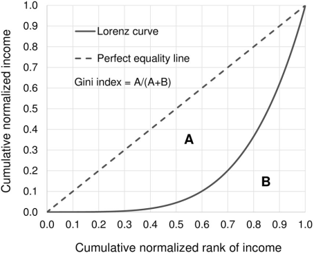
Figure 1. Illustrates the relation between Lorenz curve and GI [7].
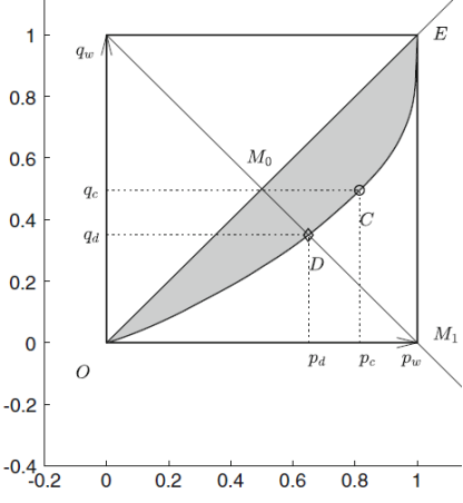
Figure 2. Lorenz curve and its characteristic points [7].
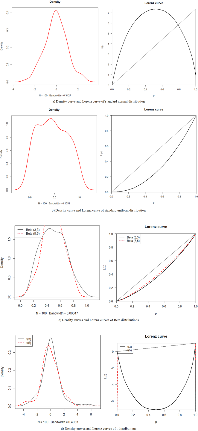
Figure 3. The density curves and Lorenz curves of symmetric distributions.
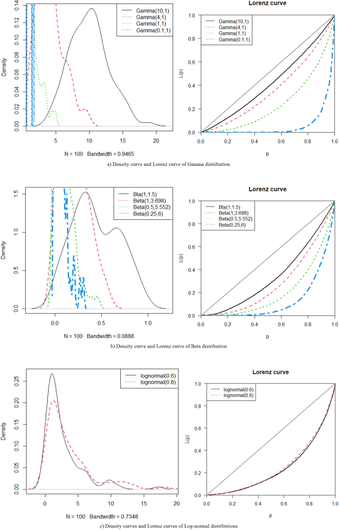
Figure 4. The density curves and Lorenz curves of positive skewed distributions.
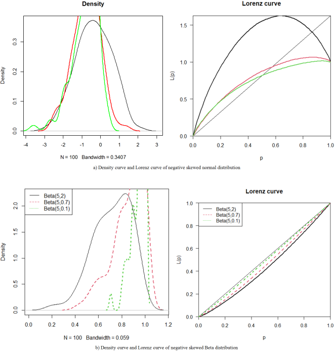
Figure 5. The density curves and Lorenz curves of negative skewed distributions.
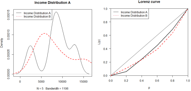
Figure 6. Density and Lorenz curves of different income distributions with the same GI.
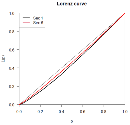
Figure 7. Plotting the Lorenz curve for distributions of the scores in the first year from section (1) and section (6).
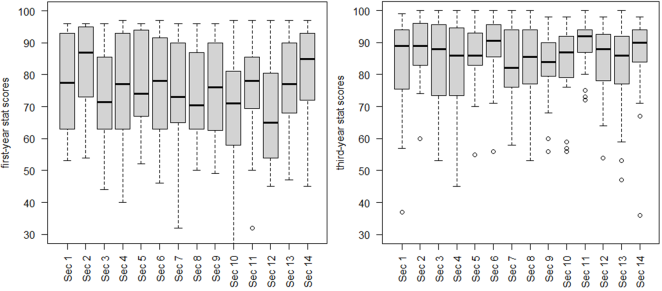
Figure 8. The boxplot shows the students' test scores from their first and third years.
Information

