Application of Lagrange Multiplier for Solving Non – Homogenous Differential Equations

Partha Sarathi Basak

doi:doi:10.11648/j.ajam.20241205.11

Research Article |

| Peer-Reviewed

Application of Lagrange Multiplier for Solving Non – Homogenous Differential Equations

Partha Sarathi Basak^*

Published in American Journal of Applied Mathematics (Volume 12, Issue 5)

Received: 1 August 2024 Accepted: 28 August 2024 Published: 11 September 2024

Views: Downloads:

Download PDF

Share This Article

Twitter
Linked In
Facebook

Abstract

The Lagrange Multiplier method has been applied in solving the regular Sturm Liouville (RSL) equation under a boundary condition of the first kind (Dirichlet boundary condition). This method is a very powerful tool for solving the RSL equation and it involves the solution of the RSL equation with the expansion of eigenfunctions into trigonometric series. The efficiency of this approach is emphasized by solving two examples of regular Sturm Liouville problem under homogenous Dirichlet boundary conditions. The methodology is effectively demonstrated, and the results show a high degree of accuracy of the solution in comparison with the exact solution and reasonably fast convergence.

Published in	American Journal of Applied Mathematics (Volume 12, Issue 5)
DOI	10.11648/j.ajam.20241205.11
Page(s)	111-117
Creative Commons	This is an Open Access article, distributed under the terms of the Creative Commons Attribution 4.0 International License (http://creativecommons.org/licenses/by/4.0/), which permits unrestricted use, distribution and reproduction in any medium or format, provided the original work is properly cited.
Copyright	Copyright © The Author(s), 2024. Published by Science Publishing Group

Keywords

Sturm Liouville Operator, Lagrange Multiplier, Eigenvalue, Eigenfunction

1. Introduction

Differential equations with suitable initial and boundary conditions are widely used to describe the physics of the problems. In order to study the physical systems, it is important to understand the differential equations and find their solutions. It is well known that in most of the practical systems, the equations are complex and do not have conventional analytical solutions

[1-4]

. In many complex linear second order differential equations, solutions are often obtained with the help of semi–analytical or numerical methods, like a series of expansion of functions

[1, 2]

. Such obtained solutions warrant in-depth understanding in the view of the physics of the problem and their application to the real problem of physical situations needs analytical study

[3-5]

. Most of the problems in physics arise in the form of boundary value problems (BVP). In this article, the solution of linear second order differential equations with BVP will be studied.

In complex situations, the solution of BVP can be easily made with the help of variational techniques. Such as unsteady state heat and mass transfer problems can be easily converted to the problem of eigenvalue one and in these cases, variational methods are very useful

[1-3]

. However, very often, variational techniques demand both homogeneous differential equations along homogenous boundary conditions. In many physical systems, homogenous boundary conditions do not prevail particularly in the case of boundary conditions of first kind or Dirichlet boundary conditions. In such situations, it is convenient to choose a suitable variable and reduce the boundary conditions into a homogeneous one. This leads to non-homogeneous differential equations with homogeneous Dirichlet boundary conditions.

In this paper, an elegant method of solving non – homogeneous differential equations with homogeneous Dirichlet boundary conditions are described by seeking a solution as an expansion of eigenfunctions. The method involves converting the second-order differential equation to the Sturm – Liouville eigenvalue problem and equating the homogeneous part of the RSL equation to a multiplier. It is also termed as Lagrange multiplier method

[2, 4-7]

. However, the application of this method and its governing rules in the field of engineering problems are not well documented in the literature. The objective of this article is to find a straight forward approach to solve the RSL equation by deriving Lagrange multipliers and evolving a generalized solution as a set of functions. In this article, the principles of Lagrange Multiplier from a variational perspective are discussed and a deep understanding of the nature of such principles along with their application to basic problems is provided.

2. The Method

It is possible to express any second order differential equation as Sturm – Liouville equation as;

L (Z) = \frac{d}{dx} (p (x) \frac{dZ}{dx}) + q (x) Z

(1)

where, L is Sturm – Liouville operator.

In practical systems, non – homogeneous Dirichlet boundary conditions can be reduced to homogeneous ones. This leads the Sturm – Liouville equation to become a non – homogeneous one and can be expressed as,

L (Z) = F (x)

(2)

It may be noted that non – homogeneous Sturm – Liouville problems may also arise when we try to solve non – homogeneous partial differential equations (PDE). This can have two parts – a general solution to the homogenous problem and a particular solution of non – homogeneous part as;

L (Z) = L (Z_{h} + Z_{p}) = L (Z_{h}) + L (Z_{p})

(3)

such that, L (Z_{h}) = 0 and L (Z_{p}) = F (x)

(4)

Any linear second order operator can be converted into an operator with self – adjointedness by carrying out following procedure. The resulting operator is referred to as a Sturm Liouville operator which is expressed as;

L = \frac{d}{dx} p (x) \frac{d}{dx} + q (x)

(5)

Putting equation (5) into equation (2), we obtain,

L (Z) = \frac{d}{dx} (p (x) \frac{dZ}{dx}) + q (x) Z = F (x)

(6)

The functions p(x), p’(x) and q(x) are assumed to be continuous in the range (x₁, x₂) and p(x) >0 on [x₁, x₂]. Thus, the Sturm – Liouville equation becomes regular (RSL) in the interval [x₁, x₂].

A general linear second order differential equation can be expressed as below,

a_{2} (x) Z^{''} + a_{1} (x) Z^{'} + a_{0} (x) Z = f (x)

(7)

Or, Z^{''} + \frac{a_{1} (x)}{a_{2} (x)} Z^{'} + \frac{a_{0} (x)}{a_{2} (x)} Z = \frac{f (x)}{a_{2} (x)}

(8)

Both sides of equation (8) are multiplied by µ(x) and the equation may be written as;

µ (x) Z^{''} + µ (x) \frac{a_{1} (x)}{a_{2} (x)} Z^{'} + µ (x) \frac{a_{0} (x)}{a_{2} (x)} Z = µ (x) \frac{f (x)}{a_{2} (x)}

(9)

The first two terms of equation (9) can be combined into an exact derivative of

{({µZ}^{'})}^{'}

if µ(x) satisfies

\frac{dµ}{dx} = µ (x) \frac{a_{1} (x)}{a_{2} (x)}

(10)

The equation (10) can be solved to obtain µ(x) as follows;

µ (x) = e^{\int (\frac{a_{1} (x)}{a_{2} (x)}) dx}

(11)

Thus, the original equation (7) can be multiplied by a factor

\frac{µ (x)}{a_{2} (x)} = \frac{1}{a_{2} (x)} e^{\int (\frac{a_{1} (x)}{a_{2} (x)}) dx}

(12)

to turn it into RSL form of equation (6). In summary, it may be expressed as follows;

p (x) = e^{\int (\frac{a_{1} (x)}{a_{2} (x)}) dx}

(13)

q (x) = p (x) \frac{a_{0} (x)}{a_{2} (x)}

(14)

and, F (x) = p (x) \frac{f (x)}{a_{2} (x)}

(15)

Hence it is possible to transform any linear second order differential equation in the form of Sturm-Liouville equation and can be described as in equation (2), where Z(x) is to satisfy given homogeneous Dirichlet boundary conditions. The eigenfunction expansion method makes use of eigenfunctions, Φ_n(x), satisfying the eigenvalue problem and can be equated with the left side of equation (2), subject to the given boundary conditions.

L (Φ_{n}) = - λσ (x) Φ_{n}

(16)

Here, λ is the Lagrange multiplier

[2, 6-10]

and σ(x) is weight function. Then Z(x) of equation (2) can be written as an expansion in the eigenfunctions such as;

Z (x) = \sum_{n = 1}^{\infty} C_{n} Φ_{n} (x)

(17)

Inserting the expansion of equation (17) into the left part of non-homogeneous differential equation (16) gives;

L (\sum_{n = 1}^{\infty} C_{n} Φ_{n} (x)) = - \sum_{n = 1}^{\infty} C_{n} λ_{n} σ (x) Φ_{n} (x)

(18)

Therefore, the non – homogeneous part of equation (2), F(x), can be expressed as a series of expansion of eigenfunctions as:

F (x) = - \sum_{n = 1}^{\infty} C_{n} λ_{n} σ (x) Φ_{n} (x)

(19)

It is known that inner product of two functions f(x) and g(x) can be defined in the interval [x₁, x₂] if the integral exists as;

< f, g > = \int_{x_{1}}^{x_{2}} f (x) g (x) dx

(20)

If Φ_m(x) is the m-th eigenfunction of series

{Φ n (x)}_{n = 1}^{\infty}

; which constitutes F(x), then the inner product in between F(x) and Φ_m(x) can be expressed by multiplying right part of equation (19) by Φ_m(x) and integrate over the range [x₁, x₂] as,

\int_{x_{1}}^{x_{2}} {F (x) Φ}_{m} (x) dx = - \sum_{n = 1}^{\infty} C_{n} λ_{n} \int_{x_{1}}^{x_{2}} Φ_{n} (x) Φ_{m} (x) σ (x) dx

(21)

Or, \int_{x_{1}}^{x_{2}} {F (x) Φ}_{m} (x) dx = - (C_{1} λ_{1} \int_{x_{1}}^{x_{2}} Φ_{1} (x) Φ_{m} (x) σ (x) dx + C_{2} λ_{2} \int_{x_{1}}^{x_{2}} Φ_{2} (x) Φ_{m} (x) σ (x) dx + . . + C_{m} λ_{m} \int_{x_{1}}^{x_{2}} Φ_{m} (x) Φ_{m} (x) σ (x) dx + \dots)

(22)

We consider the inner product of two functions F(x) and Φ_m(x) where F(x) is an expansion series as described in equation (19) and using the basis of orthogonality, it can be expressed as;

< F (x), Φ_{m} (x) > = \sum_{n = 1}^{\infty} C_{n} λ_{n} < Φ_{n} (x), Φ_{m} (x) > σ (x) = \sum_{n = 1}^{\infty} C_{n} λ_{n} < Φ_{m} (x), Φ_{m} (x) > δ_{n, m} σ (x)

(23)

Where, δ_{n, m} is the Kronecker delta and is defined as;

δ_{n, m} = \{{}_{1, n = m}^{0, n \neq m}

(24)

Therefore, applying orthogonality to equation (22), the following equation is obtained;

\int_{x_{1}}^{x_{2}} {F (x) Φ}_{m} (x) dx = - C_{m} λ_{m} \int_{x_{1}}^{x_{2}} Φ_{m} (x) Φ_{m} (x) σ (x) dx

(25)

Hence, it is possible to obtain expansion coefficient as follows;

C_{m} = - \frac{\int_{x_{1}}^{x_{2}} F (x) Φ_{m} (x) dx}{λ_{m} \int_{x_{1}}^{x_{2}} Φ_{m}^{2} (x) σ (x) dx}

(26)

3. Illustrative Example

In this section, we will present an example that has exact solution as well as an approximate solution can be computed with expansion series of eigenfunctions. We now consider a generalized non-homogeneous differential equation and try to solve it with Lagrange Multiplier method. For example, we try to solve;

\frac{d^{2} y}{d x^{2}} + ky = x

(27)

Under homogeneous Dirichlet boundary conditions;

y (0) = 0 = y (1)

(28)

It may be noted that this type of differential equation commonly arises in mechanical and electrical engineering, physics, and other fields where the behavior of dynamic systems is analyzed. It may be pointed out that application of the method of separation on unsteady state heat or mass transfer problems often leads into ordinary differential equation which are usually in the form of equation (27). In many physical problems, the above differential equation (27) relates to a mass – spring system with an external force. Solving the differential equation would provide the function y(x), giving a displacement of the mass as a function of the external force applied.

Applying equation (13), (14) and (15), it is possible to convert equation (27) to RSL form as follows:

{(y^{'})}^{'} + ky = x

(29)

Where, p(x) = 1, q(x) = k and F(x) = x.

If Φ is the set of eigenfunctions, then LHS of equation (29) can equated to Lagrange multiplier as follows:

Φ^{''} + kΦ = - λσ (x) Φ

(30)

Where, λ is Lagrange Multiplier

[2, 6, 8-10]

, σ(x) is weight function and σ(x) > 0. In this case, we consider σ(x) = 1 and rewrite the equation (30) as;

Φ^{''} + (k + λ) Φ = 0

(31)

Here, we assume λ > - k, so that the eigenfunctions become expansion series of trigonometric functions. It may be mentioned that k may a constant or a function of x. Therefore, the solution can be written as:

Φ_{n} (x) = Acos ((\sqrt{k + λ}) x) + Bsin (\sqrt{(k + λ)} x)

(32)

Putting the first part of boundary conditions (28), we obtain A = 0 and, therefore;

Bsin ((\sqrt{k + λ}) x) = 0

(33)

If B = 0, then the solution becomes trivial one. Hence, we assume,

\sin (\sqrt{(k + λ)} x) = 0

(34)

The equation (34) can lead the solution of equation (30) to some meaningful solution and the equation (34) is only valid when

λ_{n} = n^{2} π^{2} - k

. Therefore, the solution can be expressed as;

Φ_{n} (x) = Bsin (nπx)

(35)

In order to find out B, it is often useful to normalize the eigenfunctions. Thus, we have

\int_{0}^{1} {(Φ_{n} (x))}^{2} σ (x) dx = 1

(36)

Since, σ(x) = 1, the equation becomes;

\int_{0}^{1} B^{2} {(\sin (nπx))}^{2} dx = 1

(37)

Thus, we obtain

B = \sqrt{2}

and the solution becomes;

y_{n} = \sum_{n = 1}^{\infty} C_{n} Φ_{n} (x)

(38)

Now, we first expand the unknown solution in terms of eigenfunctions and equate with non – homogeneous part of equation (29).

x = - \sum_{n = 1}^{\infty} C_{n} λ_{n} (\sqrt{2}) \sin (nπx)

(39)

Applying orthogonality and equations (22) to (25) and equation (39), it can be easily derived as;

C_{m} = - \frac{\int_{0}^{1} x Φ_{m} (x) dx}{λ_{m} \int_{0}^{1} {(Φ_{m} (x))}^{2} σ (x) dx}

(40)

Since, we considered σ(x) = 1, each coefficient can easily be derived as follows:

C_{m} = - \frac{1}{\sqrt 2} \frac{\int_{0}^{1} xsin (mπx) dx}{(m^{2} π^{2} - k) \int_{0}^{1} {(\sin (mπx))}^{2} dx}

(41)

The above equations (40) and (41) is true when k is constant. If k is a function of x, then equation (41) should be rewritten as;

C_{m} = - \frac{1}{\sqrt 2} \frac{\int_{0}^{1} xsin (mπx) dx}{\int_{0}^{1} (m^{2} π^{2} - k) {(\sin (mπx))}^{2} dx}

(42)

4. Results

4.1. Analysis with Constant k

In this section, a reasonably simple form of the differential equation for the solution is chosen with constant k so that it is possible to compare the results with that of the exact solution.

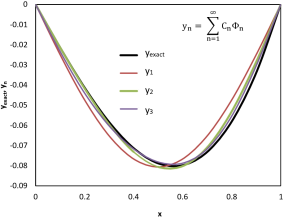
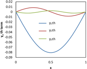
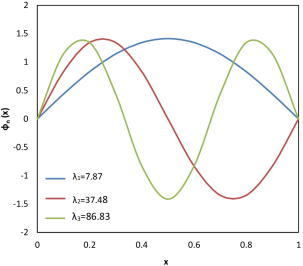
Figure 1 shows the comparison of results between the exact solution and solutions obtained from equation (38) in the interval [0, 1]. It is clear that the solution of equation (29) in the Lagrange multiplier method with even 2 terms almost matches the exact solution. The variation of each term with x is illustrated in Figure 2. Figure 3 displays the behavior of each eigenfunction by computing variations after derivation of n-th term Lagrange multiplier and shows the variational approach to estimate the solution with increasing eigenvalues

[4-6, 8-11]

Download: Download full-size image

Figure 1. Comparison of exact solution y = f(x) with solutions obtained from Lagrange Multiplier method with different number of terms computed (k = 2).

Download: Download full-size image

Figure 2. Variation y_nth term with x (k = 2).

Download: Download full-size image

Figure 3. The variation of eigenfunctions at different eigenvalues (λ_n) with x (k = 2).

4.2. Analysis with k as a Function of x

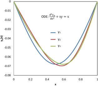
When k of equation (29) is a function of x, equation (42) should be used to determine the coefficients and solve the differential equation. We have considered k = x and the equation becomes:

\frac{d^{2} y}{d x^{2}} + xy = x

(43)

The equation (43) has been solved under the boundary condition (28) using equation (42) and the results are illustrated in figure 4.

Download: Download full-size image

Figure 4. Variation of y_n(x) with x at different number of terms when k = x.

The results are compared with one, two and three terms of Lagrange multiplier solution. It may be noted that the equation (43) under homogenous Dirichlet boundary conditions does not have exact solution. However, it is evident from the figure 4 that the solution with n = 3 approaches to desired accuracy and this will be separately emphasized in the next section.

4.3. Remarks

It should be noted that one must take a sufficiently large number of coefficients of y_n(x) so that the solution converges and approaches to very near exact value. The conditions for the convergence of the solution broadly are discussed in the literature. However, these estimates are so complicated that they are impractical in actual situations

[1, 2, 11]

. For this reason, it is convenient to calculate y_n(x) and y_n+1(x) and compare the results. If the two successive terms coincide within the limits of desired accuracy, then the solution of the variational problem can be taken as y_n(x) and the corresponding value of λ is accepted. Otherwise, further iteration process is repeated till the values agree within the desired accuracy.

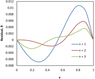
Figure 5 shows that the residual reduces as n increases when k is assumed to constant. This suggests that the residual, R, can be used as a criterion and this has been established for many problems

[1, 7, 10, 11]

R = y_{exact} - y_{n}

(44)

Download: Download full-size image

Figure 5. Residual as a function of x with (i) n = 1, (ii) n = 2, (iii) n = 3. (k = 2).

Comparing the residuals in Figure 5, it is clear that the approximate solution corresponding to the case n = 3 would be a fairly good solution. Furthermore, error bounds can often be derived in terms of residual, so that the error bounds are improved

[1, 2, 7, 10, 11]

. For all problems, one can use the residual as a guide to the success of approximation, and in many problems, this guide can be made precise with numerical values for errors. It is more difficult to establish error bounds than finding the solution.

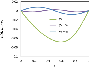
If k is a function of x, one should examine the convergence of two successive terms and justify the desired accuracy with requirement of the practical systems as exact solution of equation (43) does not exist. Figure 6 displays the difference of two consecutive terms and it is clear that the difference in between y₃ and y₂

solution becomes lesser than that of y₂ and y₁. For the requirement of very precise results, higher approximations must be calculated. As n increases, one can expect the residual become smaller.

Download: Download full-size image

Figure 6. Difference of two successive terms as a function of x (k = x). The solution with n = 3 is also displayed for comparison.

5. Conclusions

In this article, an analytical method called Lagrange multiplier method from a variational approach for a solution of non – homogeneous second order differential equation under homogeneous Dirichlet boundary condition has been presented. In this method, it is mandatory to expand eigenfunctions into the series of trigonometric functions to achieve meaningful, non – trivial and convergent solutions.

The solution of non – homogeneous second order differential equation has been obtained where an exact solution is available and therefore, it has been possible to compare the results with the exact solution. In actual physical systems, the field differential equation is much more complicated, and further complexity arises due to boundary conditions. Therefore, this method of solving non – homogeneous RSL in terms of expansion of trigonometric series has been effectively applied to the RSL problems where exact solution does not exist. In such cases, one should compare the results of two successive terms for desired accuracy and convergence. Finally, it is evident from the analysis emphasized in this article that the Lagrange multiplier method is a very powerful and reasonably easy tool for solving non – homogenous linear RSL equations with varied boundary conditions of the first kind.

Abbreviations

RSL	Regular Sturm Liouville
BVP	Boundary Value Problem

Author Contributions

Partha Sarathi Basak is the sole author. The author read and approved the final manuscript.

Data Availability Statement

The corresponding author can provide the data analysis during the current study on reasonable request.

Conflicts of Interest

The author declares no conflicts of interest.

References

[1]	Finlayson, B. A. The Method of Weighted Residuals and Variational Principles, Academic Press; 1972, New York.
[2]	Gupta, A. S. Calculus of Variations with Applications, PHI Publishing; 1997, New Delhi. ISBN: 978-81-203-1120-6.
[3]	Kot, M. Chapter 4: Basic Generalization – A First Course in Calculus of Variations; 2014, American Mathematical Society. ISBN: 978-1-4704-1495-5.
[4]	Borwein, J. M., and Zhu, Q. J. Techniques of Variational Analysis; 2005, Springer – Verlag.
[5]	Perera, U., and Bockman, C. Solutions of Sturm Liouville Problems, Mathematics. 2020, 8, p2074. http://doi.org/10.3390/math8112074
[6]	Altiman, D., and Ugur, O. Variational Iterative Method for Sturm Liouville Differential Equations, Computers and Mathematics with Applications. 2009, 58, 322-328. http://doi.org/10.1016/j.camwa.2009.02.029
[7]	Cipu, E. C., and Barbu, C. D. Variational Estimation Methods for Sturm – Liouville Problems, Mathematics. 2022, 10, 3728. http://doi.org/10.3390/math10203728
[8]	Anjum, N., and He, J-H. Laplace Transform: Making the Variational Iteration Method Easier, Appl. Math Lett. 2019, 92, 134-138. http://doi.org/10.1016/j.aml.2019.01.016
[9]	Nadeem, M., and Yao, S-W. Solving System of Partial Differential Equations using Variational Iterative Method with He’sPolynomials, J. Math. Comp. Sci. 2014, 19, 203-211. http://doi.org/10.22436/jmcs.019.03.07
[10]	Khan, M., Hassan, Q. M. U., Haq, E. U., Khan, M. Y., Ayub, K., and Ayub, J. Analytical Technique with Lagrange Multiplier for Solving Specific Nonlinear Differential Equations, J. of Science and Arts. 2021, 21, 1(54), 5-14. http://doi.org/10.46939/J.Sci.Arts-21.1-a01
[11]	Razdan, A. K., and Ravichandran, V. Fundamentals of Partial Differential Equations, Springer; 2022, Singapore.

Cite This Article

Plain Text BibTeX RIS

APA Style

Basak, P. S. (2024). Application of Lagrange Multiplier for Solving Non – Homogenous Differential Equations. American Journal of Applied Mathematics, 12(5), 111-117. https://doi.org/10.11648/j.ajam.20241205.11

Copy | Download

ACS Style

Basak, P. S. Application of Lagrange Multiplier for Solving Non – Homogenous Differential Equations. Am. J. Appl. Math. 2024, 12(5), 111-117. doi: 10.11648/j.ajam.20241205.11

Copy | Download

AMA Style

Basak PS. Application of Lagrange Multiplier for Solving Non – Homogenous Differential Equations. Am J Appl Math. 2024;12(5):111-117. doi: 10.11648/j.ajam.20241205.11

Copy | Download

@article{10.11648/j.ajam.20241205.11,
  author = {Partha Sarathi Basak},
  title = {Application of Lagrange Multiplier for Solving Non – Homogenous Differential Equations
},
  journal = {American Journal of Applied Mathematics},
  volume = {12},
  number = {5},
  pages = {111-117},
  doi = {10.11648/j.ajam.20241205.11},
  url = {https://doi.org/10.11648/j.ajam.20241205.11},
  eprint = {https://article.sciencepublishinggroup.com/pdf/10.11648.j.ajam.20241205.11},
  abstract = {The Lagrange Multiplier method has been applied in solving the regular Sturm Liouville (RSL) equation under a boundary condition of the first kind (Dirichlet boundary condition). This method is a very powerful tool for solving the RSL equation and it involves the solution of the RSL equation with the expansion of eigenfunctions into trigonometric series. The efficiency of this approach is emphasized by solving two examples of regular Sturm Liouville problem under homogenous Dirichlet boundary conditions. The methodology is effectively demonstrated, and the results show a high degree of accuracy of the solution in comparison with the exact solution and reasonably fast convergence.
},
 year = {2024}
}

Copy | Download

TY  - JOUR
T1  - Application of Lagrange Multiplier for Solving Non – Homogenous Differential Equations

AU  - Partha Sarathi Basak
Y1  - 2024/09/11
PY  - 2024
N1  - https://doi.org/10.11648/j.ajam.20241205.11
DO  - 10.11648/j.ajam.20241205.11
T2  - American Journal of Applied Mathematics
JF  - American Journal of Applied Mathematics
JO  - American Journal of Applied Mathematics
SP  - 111
EP  - 117
PB  - Science Publishing Group
SN  - 2330-006X
UR  - https://doi.org/10.11648/j.ajam.20241205.11
AB  - The Lagrange Multiplier method has been applied in solving the regular Sturm Liouville (RSL) equation under a boundary condition of the first kind (Dirichlet boundary condition). This method is a very powerful tool for solving the RSL equation and it involves the solution of the RSL equation with the expansion of eigenfunctions into trigonometric series. The efficiency of this approach is emphasized by solving two examples of regular Sturm Liouville problem under homogenous Dirichlet boundary conditions. The methodology is effectively demonstrated, and the results show a high degree of accuracy of the solution in comparison with the exact solution and reasonably fast convergence.

VL  - 12
IS  - 5
ER  -

Copy | Download

Author Information

Partha Sarathi Basak

Gradient Wire Products Pvt Ltd, Howrah, India

Research Fields: Diffusion in metals, Phase transformation, Variational Calculus, Differential equations, Electrochemistry

Contact Email

http://orcid.org/0000-0001-8867-2685

Download PDF

Plain Text BibTeX RIS

APA Style

Basak, P. S. (2024). Application of Lagrange Multiplier for Solving Non – Homogenous Differential Equations. American Journal of Applied Mathematics, 12(5), 111-117. https://doi.org/10.11648/j.ajam.20241205.11

Copy | Download

ACS Style

Basak, P. S. Application of Lagrange Multiplier for Solving Non – Homogenous Differential Equations. Am. J. Appl. Math. 2024, 12(5), 111-117. doi: 10.11648/j.ajam.20241205.11

Copy | Download

AMA Style

Basak PS. Application of Lagrange Multiplier for Solving Non – Homogenous Differential Equations. Am J Appl Math. 2024;12(5):111-117. doi: 10.11648/j.ajam.20241205.11

Copy | Download

@article{10.11648/j.ajam.20241205.11,
  author = {Partha Sarathi Basak},
  title = {Application of Lagrange Multiplier for Solving Non – Homogenous Differential Equations
},
  journal = {American Journal of Applied Mathematics},
  volume = {12},
  number = {5},
  pages = {111-117},
  doi = {10.11648/j.ajam.20241205.11},
  url = {https://doi.org/10.11648/j.ajam.20241205.11},
  eprint = {https://article.sciencepublishinggroup.com/pdf/10.11648.j.ajam.20241205.11},
  abstract = {The Lagrange Multiplier method has been applied in solving the regular Sturm Liouville (RSL) equation under a boundary condition of the first kind (Dirichlet boundary condition). This method is a very powerful tool for solving the RSL equation and it involves the solution of the RSL equation with the expansion of eigenfunctions into trigonometric series. The efficiency of this approach is emphasized by solving two examples of regular Sturm Liouville problem under homogenous Dirichlet boundary conditions. The methodology is effectively demonstrated, and the results show a high degree of accuracy of the solution in comparison with the exact solution and reasonably fast convergence.
},
 year = {2024}
}

Copy | Download

TY  - JOUR
T1  - Application of Lagrange Multiplier for Solving Non – Homogenous Differential Equations

AU  - Partha Sarathi Basak
Y1  - 2024/09/11
PY  - 2024
N1  - https://doi.org/10.11648/j.ajam.20241205.11
DO  - 10.11648/j.ajam.20241205.11
T2  - American Journal of Applied Mathematics
JF  - American Journal of Applied Mathematics
JO  - American Journal of Applied Mathematics
SP  - 111
EP  - 117
PB  - Science Publishing Group
SN  - 2330-006X
UR  - https://doi.org/10.11648/j.ajam.20241205.11
AB  - The Lagrange Multiplier method has been applied in solving the regular Sturm Liouville (RSL) equation under a boundary condition of the first kind (Dirichlet boundary condition). This method is a very powerful tool for solving the RSL equation and it involves the solution of the RSL equation with the expansion of eigenfunctions into trigonometric series. The efficiency of this approach is emphasized by solving two examples of regular Sturm Liouville problem under homogenous Dirichlet boundary conditions. The methodology is effectively demonstrated, and the results show a high degree of accuracy of the solution in comparison with the exact solution and reasonably fast convergence.

VL  - 12
IS  - 5
ER  -

Copy | Download